Differential Equations
Mathwrist Code Example Series

Copyright ©Mathwrist LLC 2023
(October 5, 2023)
Abstract

This document gives some code examples on how to use differential equation solvers in Mathwrist’s C++ Numerical Programming Library (NPL).

1 HIRES Benchmark Problem

The HIRES benchmark test problem refers to “High Irradiance RESponse”. It originates from plant physiology and describes how light is involved in morphogenesis. It is a stiff nonlinear ODE system of 8 equations,

y(t)=f(y),0tT,T=321.8122,
y(0)=(1,0,0,0,0,0,0,0.0057)T
f(y)=(-1.71y0+0.43y1+8.32y2+0.00071.71y0-8.75y1-10.03y2+0.43y3+0.035y48.32y1+1.71y2-1.12y3-1.745y4+0.43y5+0.43y6-280y5y7+0.69y3+1.71y4-0.43y5+0.69y6280y5y7-1.81y6-280y5y7+1.81y6)

The solution at T=321.8122 is,

y(T)=(0.7371312573325668e-30.1442485726316185e-30.5888729740967575e-40.1175651343283149e-20.2386356198831331e-20.6238968252742796e-20.2849998395185769e-20.2850001604814231e-2)
1 // Derive under the general ODE interface
2 struct Hires : public ODE
3 {
4    size_t size() const { return 8; }
5    double start_time() const { return 0; }
6    double end_time() const { return  321.8122; }
8    // Implement y’(t) = f(t,y)
9    void y_prime(double, const double* y, double* f) const
10    {
11       f[0] = -1.71 * y[0] + 0.43 * y[1] + 8.32 * y[2] + 0.0007;
12       f[1] = 1.71 * y[0] - 8.75 * y[1];
13       f[2] = -10.03 * y[2] + 0.43 * y[3] + 0.035 * y[4];
14       f[3] = 8.32 * y[1] + 1.71 * y[2] - 1.12 * y[3];
15       f[4] = -1.745 * y[4] + 0.43 * y[5] + 0.43 * y[6];
16       f[5] = -280 * y[5] * y[7] + 0.69 * y[3] + 1.71 * y[4] -
17          0.43 * y[5] + 0.69 * y[6];
18       f[6] = 280 * y[5] * y[7] - 1.81 * y[6];
19       f[7] = -280 * y[5] * y[7] + 1.81 * y[6];
20    }
21 };
23 // Create an object of the ODE problem
24 Hires hires;
26 // Initial value
27 double y0[8] = { 1, 0, 0, 0, 0, 0, 0, 0.0057 };
29 // Final solution
30 double yT[8] =
31 {
32    0.7371312573325668e-3,
33    0.1442485726316185e-3,
34    0.5888729740967575e-4,
35    0.1175651343283149e-2,
36    0.2386356198831331e-2,
37    0.6238968252742796e-2,
38    0.2849998395185769e-2,
39    0.2850001604814231e-2
40 };
42 // Create the solver using spectral IDeC explicit method,
43 // degree of interpolation polynomial = 7,
44 // number of error correction iteration = 3
45 ODE_IDeC idec(ODE_IDeC::O1_SPECTRAL_EXPLICIT, 7, 3);
47 // solve the problem with N number of time steps
48 const int N = 100000;
49 idec(hires, N, y0, y0);
51 // Check the result
52 for (int i = 0; i < 8; ++i)
53 {
54    double error = y0[i] - yT[i];
55    ftl::Assert(std::abs(error) < 3.e-12);
56 }

Since the HIRES problem is nonlinear, at line 2 we create a struct Hires derived from NPL’s general ODE interface class ODE. Lines 4 to 6 implement base class virtual functions to specify the ODE’s size, start and end time. We supply an implementation of the y_prime virtual function from line 9 to 20 to compute y(t).

At line 45, we create an IDeC solver to use 𝒪(h) explicit base method and spectral IDeC. We further instruct IDeC to use an approximation polynomial of degree 7 and 3 error correction iterations. On a laptop with 2.60GHz CPU and 8.00 GB RAM, this problem is solved in less than 0.02 seconds with absolute error tolerance smaller than 3.e-12. In comparable time and machine setup, this result is 2 order more accurate than the benchmark result on SciML Benchmark and Test Set for IVP Solvers.

2 An Example of Linear ODE

This is an example of linear ODE to demonstrate NPL’s implicit IDeC method. The problem is defined as the following:

y(t)=(3124)y+(eαt0), with y(0)=(00)

It has an analytic solution

y(t)=23eαt-e2tα-2v1+13eαt-e5tα-5v2,
v1=(1-1)v2=(12)
1 // Derive from linear ODE interface
2 struct O : public ODE_Linear
3 {
4    double m_alpha;
5    double m_T;
6    O(double alpha, double T) : m_alpha(alpha), m_T(T) {}
8    size_t size() const { return 2; }
9    bool homogeneous() const { return false; }
10    double start_time() const { return 0; }
11    double end_time() const { return m_T; }
12    size_t size_A() const { return 0; }
14    // Compute y’(t) = f(t,y(t))
15    void y_prime(double t, const double* y, double* f) const
16    {
17       double x0 = y[0];
18       double x1 = y[1];
20       f[0] = 3 * x0 + x1 + std::exp(m_alpha * t);
21       f[1] = 2 * x0 + 4 * x1;
22    }
24    // Compute A(t) and s(t)
25    // Here A(t) is a constant 2 x 2 matrix. We decide to store
26    // it inside the ODE internally. So the second parameter
27    // is ignored. We only update s(t) here.
28    void update(double t, double*, double* s) const
29    {
30       s[0] = std::exp(m_alpha * t);
31       s[1] = 0;
32    }
34    // Solve 2 by 2 linear system (I - h A(t)) y = rhs
35    // Again since A(t) is constant, the first and second
36    // parameters are ignored.
37    void solve(const double*, double, double h, double* _y) const
38    {
39       double r0 = _y[0];
40       double r1 = _y[1];
42       double a = 1 - 3 * h;
43       double b = -h;
44       double c = -2 * h;
45       double d = 1 - 4 * h;
47       _y[1] = (c * r0 - a * r1) / (b * c - a * d);
48       _y[0] = (r0 - b * _y[1]) / a;
49    }
51    // Compute y’(t) = A(t) y(t) + s(t)
52    void Ays(const double*, const double* _y, const double* s,
53       double* _yp) const
54    {
55       double x0 = _y[0];
56       double x1 = _y[1];
58       _yp[0] = 3 * x0 + x1 + s[0];
59       _yp[1] = 2 * x0 + 4 * x1;
60    }
61 };
63 // First coefficient term of the analytic solution
64 auto coeff_1 = [](double alpha, double t)
65 {
66    return 2./3. * (std::exp(alpha * t) - std::exp(2 * t))/(alpha - 2);
67 };
69 // Second coefficient term of the analytic solution
70 auto coeff_2 = [](double alpha, double t)
71 {
72    return 1./3. * (std::exp(alpha * t) - std::exp(5 * t))/(alpha - 5);
73 };
75 // Create an object of the ODE problem
76 double T = 1;
77 double alpha = 0.05;
78 O ode(alpha, T);
80 double u[2] = { 0, 0 };
81 double y0[2] = { 0, 0 };
82 double yT[2] = { 0, 0 };
84 double c1 = coeff_1(alpha, T);
85 double c2 = coeff_2(alpha, T);
87 yT[0] = c1 + c2;
88 yT[1] = -c1 + 2 * c2;
90 // Number of time steps
91 const int N = 2000;
93 // Create a solver to use classic implicit IDeC method.
94 // Interpolation polynomial degree = 6,
95 // Number of error correction iterations = 3.
96 ODE_IDeC idec(ODE_IDeC::O1_CLASSIC_IMPLICIT, 6, 3);
97 idec(ode, N, y0, y0);
99 // Check the result
100 ftl::Assert(std::abs(y0[0] - yT[0]) < 1.e-8);
101 ftl::Assert(std::abs(y0[1] - yT[1]) < 1.e-8);

At line 2, we now derive from NPL’s linear ODE interface ODE_Linear and define the behavior of this ODE via a set of virtual functions. For large linear ODE systems, A(t) often is a sparse matrix. NPL allows users to store A(t) in a user-designed compact form. The size_A virtual function is used by IDeC solvers to allocate correct memory storage for matrix A(t). In this particular example though, A(t) is a constant 2×2 matrix. We let the size_A() function return 0 at line 12. This instructs IDeC solvers not to allocate memory to store A(t).

From line 15 to 22, we supply an implementation to compute y(t). This is a virtual function indirectly inherited from the ODE base class. In addition, we also need implement virtual functions directly inherited from ODE_Linear class. Line 28 to 32 is the implementation to compute A(t) and s(t) as of time t. Because we have instructed IDeC solvers that A(t) has 0 size, a nullptr will be passed from the solver to the second parameter of the update function. We ignore this parameter and only compute s(t). Similarly, if the ODE is homogeneous, IDeC will pass nullptr to the third parameter of update function.

From line 37 to 49, we solve an linear system (𝐈-h𝐀(t))𝐲=𝐫 for some right hand side (rhs) vector 𝐫. It is users’ responsibility to solve this equation based on their choice of the compact form of A(t). Again, because A(t) is not stored at IDeC solver side, the first parameter passed to this function is a nullptr. Since A(t) is constant here, we also ignore the second parameter t in this function. The function body simply inverts the system and save result back to buffer pointer _y.

Lastly, line 52 to 60 computes y(t)=A(t)y(t)+s(t) using a pointer to the compact storage of A(t), which is a nullptr here as we explained. Pointer s will be nullptr for homogeneous system. Two Lambda functions at line 64 and 70 are the coefficient terms of the analytic solution y(t). At line 96, we create a classic IDeC solver using interpolation polynomial of degree 6 and 3 number of error iterations. Because of the stability of implicit methods, we are able to solve the problem with a relatively large time step size.

3 PDE - Heat Equations

In this example we have 2 unknown functions v1(t,x) and v2(t,x) that are governed by the same PDE and Dirichlet boundary conditions,

vt=142vx2,x(0,2),t(0,1)
v(t,0)=0,v(t,2)=0

They differ from each other on the following initial values

v1(0,x) = 6sin(πx)
v2(0,x) = 2sin(πx2)-sin(πx)+4sin(2πx)

, and have the analytic solutions

v1(t,x) = 6sin(πx)e-π24
v2(t,x) = 2sin(πx2)e-π216-sin(πx)e-π24+4sin(2πx)e-π2

We will create different solvers to solve v1(t,x) and v2(t,x) simultaneously.

1 // Heat equation:
2 // \frac{\partial v}{\partial t}=1/4 \frac{\partial^2 v}{\partial x^2}
3 // t \in (0, T)
4 struct Heat : public PDEParabolic1D
5 {
6    Heat(double x_min, double x_max, double T) :
7       PDEParabolic1D(Bound(x_min, x_max), Bound(0, T)) {}
9    void coefficient(
10       double,
11       const double*,
12       size_t n_x,
13       double* _ftx,
14       double* /* _gtx */,
15       double* /* _htx */ ) const
16    {
17       std::fill(_ftx, _ftx + n_x, 0.25);
18    }
19 };
21 // Solve 2 initial values of heat equation simultaneously:
22 // 1) v(x, t=0)=6 sin(\pi * x);
23 // 2) v(x, t=0)=2 sin(\pi / 2 * x)-sin(\pi * x)+4 sin(2 * \pi * x);
24 struct F0 : public PDEParabolic1D::InitialValueFunct
25 {
26    void eval(const ftl::Buffer<double>& x, double t, int, Matrix& v_x) const
27    {
28       ftl::Assert(t == 0, ftl::LogicError());
29       ftl::Assert(v_x.row_size() == 2, ftl::LogicError());
31       const size_t n = x.size();
32       for (size_t ix = 0; ix < n; ix++)
33       {
34          double pi_x = PI() * x[ix];
36          // Initial values of the first problem,
37          v_x(0, ix) = 6 * std::sin(pi_x);
39          // Initial values of the second problem,
40          v_x(1, ix) = 2 * std::sin(0.5 * pi_x) - std::sin(pi_x) +
41             4 * std::sin(2 * pi_x);
42       }
43    }
44 };
46 // Analytic solution of the first problem.
47 struct F1
48 {
49    double max_error(
50       const mathwrist::ftl::Buffer<double>& x,
51       const mathwrist::Matrix& V_pde) const
52    {
53       double error = 0;
54       size_t n_x = x.size();
55       for (size_t i = 0; i < n_x; i++)
56       {
57          double pi_x = PI() * x[i];
58          double v1 = 6 * std::sin(pi_x) * std::exp(-0.25 * PI() * PI());
59          double v2 = V_pde(0, i);
60          error = std::max(error, std::abs(v1 - v2));
61       }
63       return error;
64    }
65 };
67 // Analytic solution of the second problem.
68 struct F2
69 {
70    double max_error(
71       const mathwrist::ftl::Buffer<double>& x,
72       const mathwrist::Matrix& V_pde) const
73    {
74       double error = 0;
75       size_t n_x = x.size();
76       for (size_t i = 0; i < n_x; i++)
77       {
78          double pi_2 = PI() * PI();
79          double pi_x = PI() * x[i];
80          double v1 = 2 * std::sin(0.5*pi_x) * std::exp(-pi_2 / 16.0)
81             - std::sin(pi_x) * std::exp(-pi_2 / 4.0)
82             + 4 * std::sin(2 * pi_x) * std::exp(-pi_2);
83          double v2 = V_pde(0, i);
84          error = std::max(error, std::abs(v1 - v2));
85       }
87       return error;
88    }
89 };
91 // Test domain: x \in (0, 2), t \in (0, 1)
92 const double T = 1;
93 const double x_lo = 0;
94 const double x_hi = 2;
95 Heat heat(x_lo, x_hi, T);
97 // boundary condition v(0) = v(2) = 0 for both problems.
98 struct BC : public PDEParabolic1D::BoundaryCondition
99 {
100    BC() : PDEParabolic1D::BoundaryCondition(1, 0) {}
101    double eval(double, double, size_t) const { return 0; }
102 };
104 F0 f0;
105 F1 f1;
106 F2 f2;
107 BC bc_lo, bc_hi;
109 // For comparison purpose, using the same time discretizatin step.
110 const double dt = 0.001;
111 const double dx = 0.001;
113 PDEParabolic1D::Specification spec;
114 spec.n_problems = 2; // solve 2 problems together
116 // Crank-Nicolson method
117 {
118    PDEParabolic_CN pde_fd(heat, dx, dt);
120    Matrix vx;
121    pde_fd(F0(), bc_lo, bc_hi, 0, spec, vx);
123    const ftl::Buffer<double>& x = pde_fd.states();
124    const size_t J = x.size() - 1;
126    // Test max error
127    double error_1 = f1.max_error(x, vx.row(0));
128    double error_2 = f2.max_error(x, vx.row(1));
130    ftl::Assert(error_1 < 1.e-6);
131    ftl::Assert(error_2 < 1.e-6);
132 }
134 // 2nd order method of lines
135 {
136    PDEParabolic_MoL mol(heat, PDEParabolic_MoL::O2, 3, dx, dt);
138    Matrix vx;
139    mol(F0(), bc_lo, bc_hi, 0, spec, vx);
141    const ftl::Buffer<double>& x = mol.states();
143    double error_1 = f1.max_error(x, vx.row(0));
144    double error_2 = f2.max_error(x, vx.row(1));
146    ftl::Assert(error_1 < 1.1e-6);
147    ftl::Assert(error_2 < 1.e-6);
148 }
149 // 4-th order method of lines
150 {
151    PDEParabolic_MoL mol(heat, PDEParabolic_MoL::O4, 3, dx, dt);
153    Matrix vx;
154    mol(F0(), bc_lo, bc_hi, 0, spec, vx);
156    const ftl::Buffer<double>& x = mol.states();
158    double error_1 = f1.max_error(x, vx.row(0));
159    double error_2 = f2.max_error(x, vx.row(1));
161    ftl::Assert(error_1 < 1.e-10);
162    ftl::Assert(error_2 < 1.e-10);
163 }
164 // Spectral collocation method
165 {
166    int degree = 11;
167    PDEParabolic_SC pde_sc(heat, degree, 3, dt);
169    Matrix C;
170    pde_sc(f0, bc_lo, bc_hi, 0, spec, C);
172    // Numerical solution of the first problem represented
173    // by a Chebyshev curve.
174    ChebyshevCurve cheby1(x_lo, x_hi, degree);
175    cheby1.set_basis_coeff(C.row(0));
177    // Numerical solution of the second problem represented
178    // by a Chebyshev curve.
179    ChebyshevCurve cheby2(x_lo, x_hi, degree);
180    cheby2.set_basis_coeff(C.row(1));
182    // Populate numerical solutions from Chebyshev approximation
183    // polynomial and compare to analytic solution.
184    int N = 100;
185    const double dx = (x_hi - x_lo) / N;
186    ftl::Buffer<double> x(N + 1);
187    Matrix v_pde(2, N + 1);
189    for (int i = 0; i <= N; ++i)
190    {
191       x[i] = x_lo + i * dx;
192       v_pde(0, i) = cheby1.eval(x[i]);
193       v_pde(1, i) = cheby2.eval(x[i]);
194    }
196    double error_1 = f1.max_error(x, v_pde.row(0));
197    double error_2 = f2.max_error(x, v_pde.row(1));
199    // The given 2 problems have very oscillating initial values,
200    // which is not "smooth" enough for just a few collocation
201    // points to represent the function. The numerical error is
202    // relatively large.
203    //
204    // Chebyshev collocation method outperforms when v(t,x) is very
205    // smooth.
206    ftl::Assert(error_1 < 1.e-6);
207    ftl::Assert(error_2 < 1.5e-5);
208 }

At line 4, we create a derived struct Heat under the PDEParabolic1D interface. From line 9 to 18, we implement the coefficient pure virtual function by filling the f(t,x) coefficient buffer with constant 14. Since we don’t have other coefficient terms in the PDE, we ignore the _gtx and _htx buffer pointer parameters.

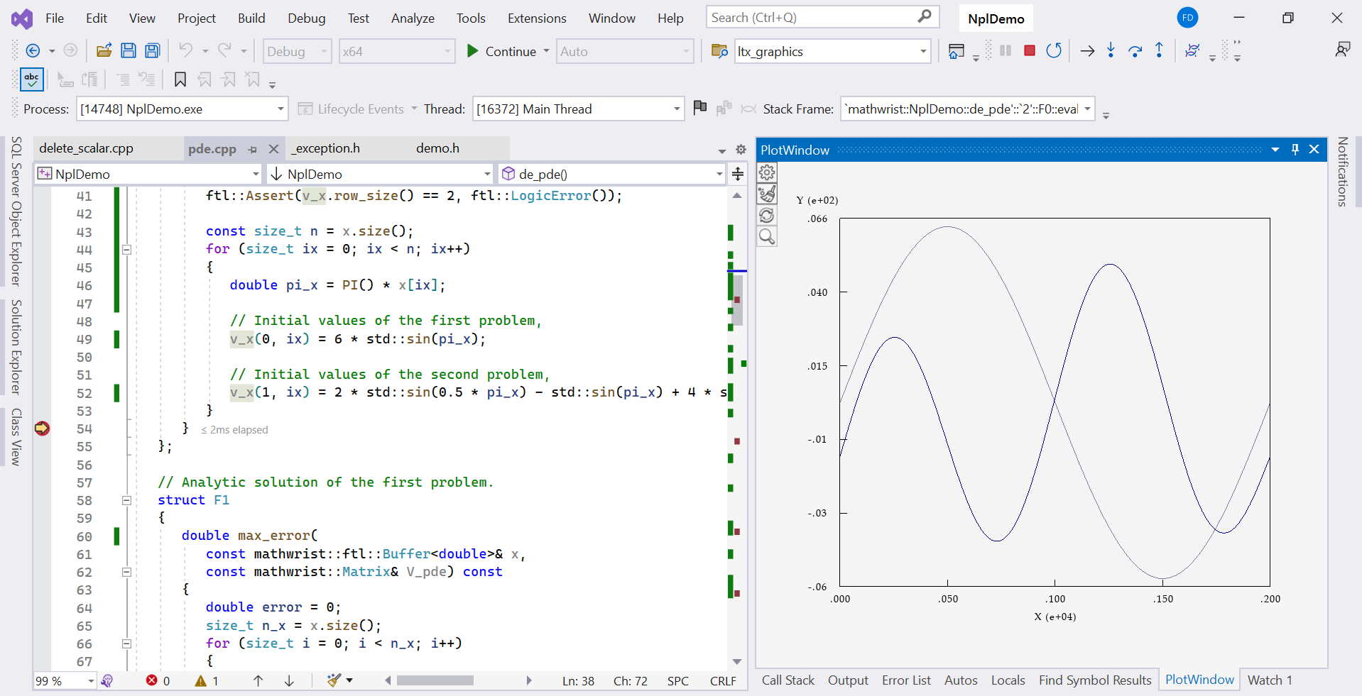
Struct F0 from line 24 to 44 implements the initial value function interface and fill v1(0,x) and v2(0,x) to 2 rows of the matrix parameter v_x in eval function. A plot of initial values can be viewed from GDE plot window illustrated in Figure 1. Struct F1 and F2 implement the analytic solution of v1(t,x) and v2(t,x) respectively.

Initial Values
Figure 1: Initial Values v1(0,x) and v2(0,x)

Between line 98 and 102, we implement the Dirichlet boundary condition. Line 113 and 114 create a PDE problem specification object, where we specify that there are 2 problems to be solved together. Code block 117 to 132 uses Crank-Nicolson method. The numerical solutions are stored in 2 separate rows of the vx matrix parameter on return. We then check the solution error from line 127 to 131.

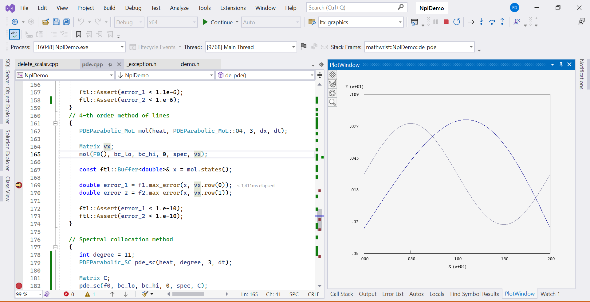
Code blocks from line 135 to 163 use the method of lines with the 2nd order finite difference scheme and the 4th order finite difference scheme. In each case, we use 3 iterations of error correction in implicit IDeC method. The 2nd order method obtains similar result as the Crank-Nicolson method. The 4th order method on the other hand produces 1.e4 times more accurate result. Figure 2 is a plot of the final numerical solutions.

Numerical Solutions of
Figure 2: Numerical Solutions of v1(t,x) and v2(t,x)

Finally code block between line 165 and 206 illustrates the spectral collocation method, where we choose Chebyshev approximation polynomial of degree 11 and 3 error correction iterations. Note that the output matrix C at line 170 consists of two rows of Chebyshev basis coefficients. We need construct 2 Chebyshev approximation polynomials with these coefficients at line 175 and 180 in order to compute the actual numerical solutions. Code block 182 to 197 uses these two approximation polynomials to evaluate the maximum numerical error over 100 discrete points. As we can see from Figure 1, the initial values are very oscillating. Chebyshev collocation method is not a good choice for this situation. Not surprisingly, Chebyshev collocation method produces large error for not very smooth functions.