GDE Surface Plots
Mathwrist User Guide Series

(October 13, 2023)

Abstract

This document is a user guide of using Mathwrist’s Graphical Debugging Extension (GDE) tool to visualize surfaces, 3-d scatter data points and NPL math objects in Microsoft Visual Studio IDE. NPL is Mathwrist’s C++ numerical programming library. 3-d functions defined in NPL are directly recognized as plottable types in GDE. Please refer to our NPL documentation series for details. For an overview of GDE, please refer to our “GDE Overview” user guide.

1 Introduction

In this document, we focus on the GDE “Surface Session” and give details on plotting 3-d scatter data points, impose a smooth surface fit to these data points and directly visualizing NPL 3-d math objects. It is recommended to read our “GDE Overview” user guide first to have a high level understanding of GDE.

Same as the curve data that we discussed in “GDE Curve Plots” user guide, surface data is represented by a matrix object with either 3 rows or 3 columns in order to be displayed in GDE surface session. The matrix type needs be a user-defined data type exported to GDE through the “mathwrist.gde.spec.json” specification json file. In the next section, we will work on a walkthrough example again to illustrate how surface plots are supported in GDE.

When NPL is used in a user’s application, NPL matrix class mathwrist::Matrix, matrix views mathwrist::Matrix::View and mathwrist::Matrix::ViewConst are recognized as user-defined matrix types. NPL 3-row and 3-column matrix objects can be plotted as 3-d scatter points. Moreover, many concrete surface types defined in NPL can be added to GDE surface session for plotting.

2 Walkthrough Example

In this code example Listing 1, we populated total 45 number of $(x,y,z)$ artificial data points to a Matrix object xyz. As we discussed in the GDE user guide series, this matrix class is defined in GDE’s demo project and imported to GDE by a plottable specification json file.

The $x$ and $y$ values are taken from some fixed coordinate points from line 13 to 16 and from line 19 to 22. The $z$ coordinate is pre-computed as $z=\sin(x^{2})\times e^{y^{2}}+\epsilon$ for some random noisy $\epsilon$ and hard-coded from line 25 to 36. Then starting from line 38 to 45, we save the $(x,y,z)$ coordinate values to matrix object xyz. Finally, we want to set a break point at line 50 and stop there to visualize the matrix object xyz.

Listing 1: Surface Plot Example

2 #include <iostream>

3 #include "demo.h"

5 void mathwrist::GDEDemo::surface()

6 {

7 // surface plot example

8 const static size_t N_POINTS = 45;

10 Matrix xyz(N_POINTS, 3);

11 {

12 // Fixed x coordinates.

13 const static double x[5] =

14 {

15 0.1, 0.3, 0.5, 0.7, 0.9

16 };

18 // Fixed y coordinates.

19 const static double y[9] =

20 {

21 0.05, 0.25, 0.35, 0.45, 0.55, 0.65, 0.75, 0.85, 0.95

22 };

24 // noisy data points f(x,y) = sin(x*x)*exp(y*y) + noise

25 const static double z[N_POINTS] =

26 {

27 0.048472, 0.022372, -0.013852, -0.032217, 0.036917,

28 0.011262, 0.011222, -0.012732, 0.039913, 0.085715,

29 0.124023, 0.150644, 0.153834, 0.166084, 0.130440,

30 0.107904, 0.145837, 0.260826, 0.231057, 0.237960,

31 0.247114, 0.271902, 0.359570, 0.393912, 0.439211,

32 0.520845, 0.652111, 0.516872, 0.480062, 0.576369,

33 0.564255, 0.594664, 0.709505, 0.838155, 0.923273,

34 1.136944, 0.752593, 0.811029, 0.825487, 0.851604,

35 0.991648, 1.084291, 1.268010, 1.467474, 1.784671

36 };

38 for (size_t k = 0; k < N_POINTS; k++)

39 {

40 size_t i = k / 9;

41 size_t j = k % 9;

42 xyz(k, 0) = x[i];

43 xyz(k, 1) = y[j];

44 xyz(k, 2) = z[k];

45 }

47 // Set a break point here, right click variable name "xyz"

48 // in a debugger and then choose to plot scatter points

49 // with fit.

50 std::cout << "done demo case: surface" << std::endl;

51 }

52 }

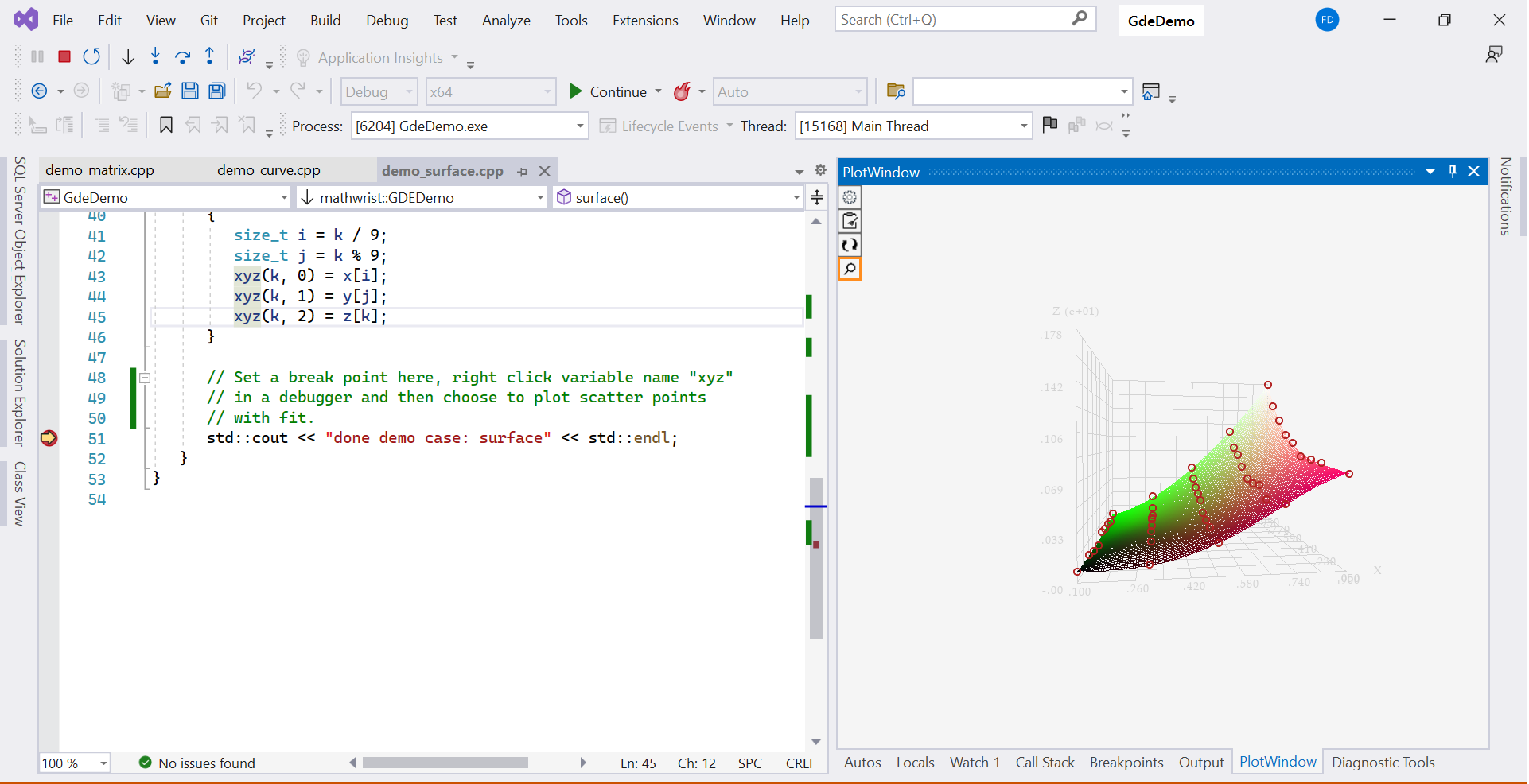
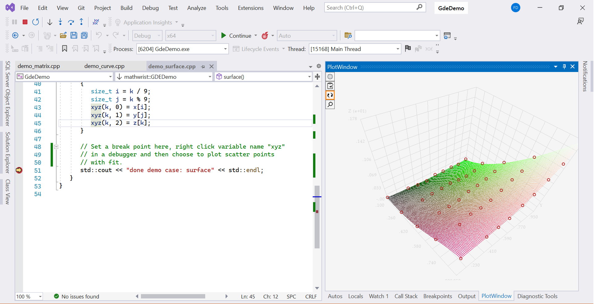
Since object xyz is a 3-column matrix, GDE is able to interpret each row of xyz as a 3-d scatter data point. Therefore, when we stop at the break point at line 50 in a debug session, right clicking variable name xyz and then clicking “plot xyz” context menu command will trigger a display choice popup window as Figure 1.

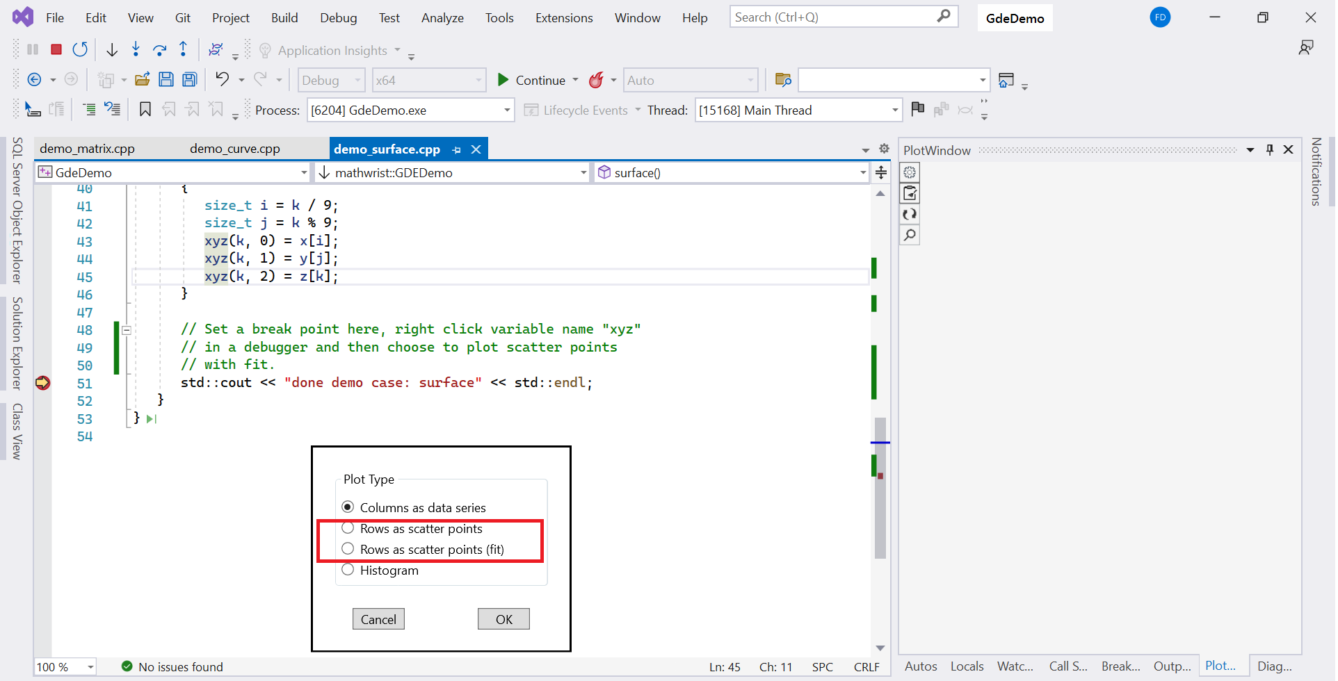
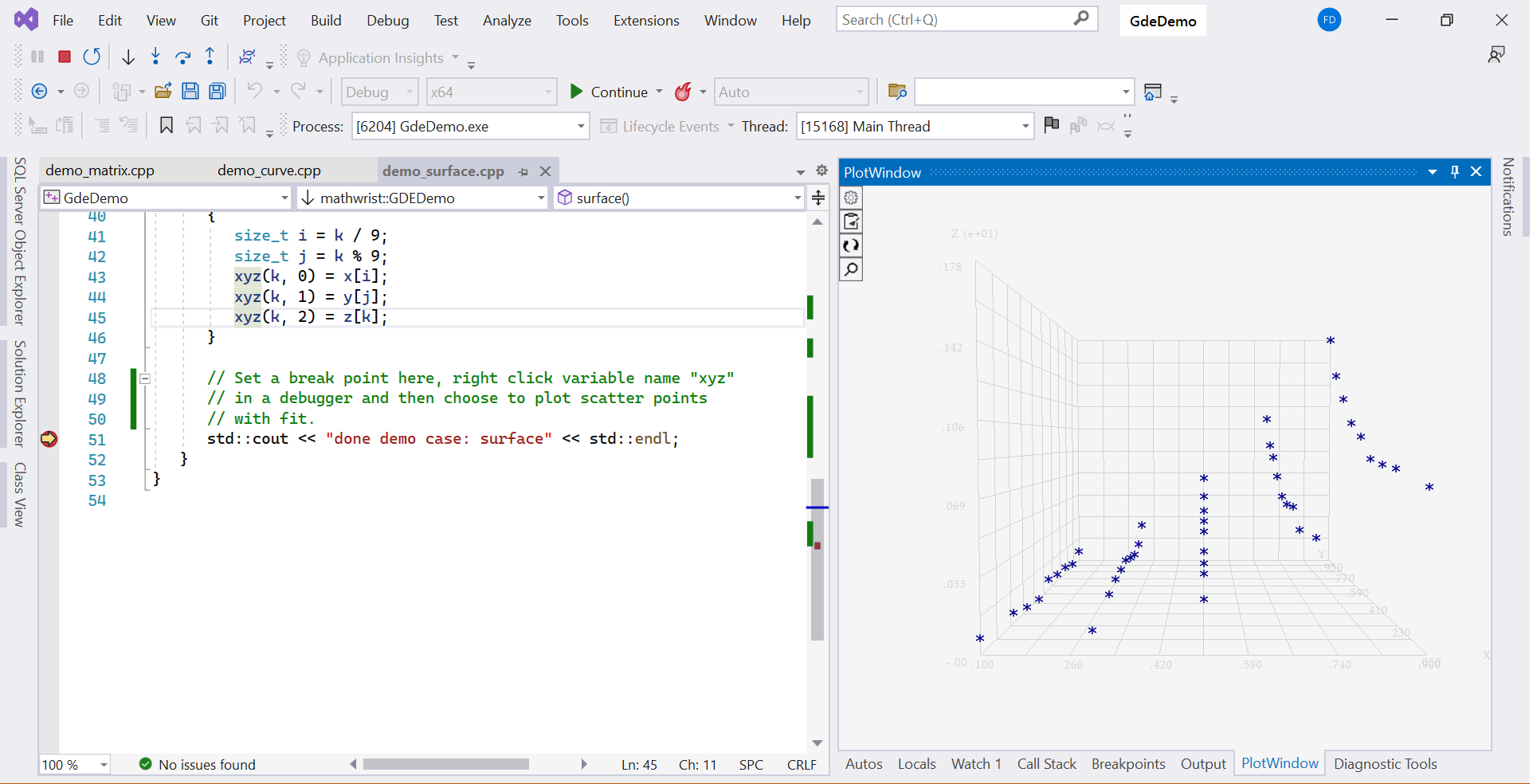
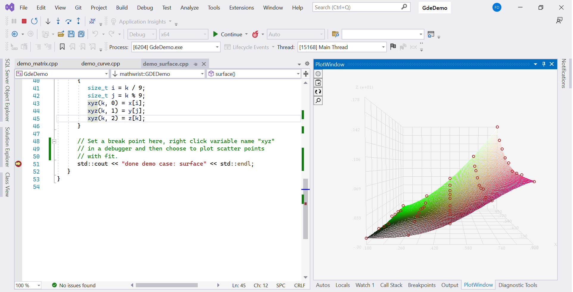
Two radio button choices “Rows as scatter points” and “Rows as scatter points (fit)” are circled in the red rectangle in Figure 1 for plotting the 3-d scatter data points alone and plotting them together with a smooth surface fit. The finaly display for each radio button choice is illustrated in figure 2(a) and 2(b).

3 Rotation and Zooming

Once the GDE surface session becomes to the active session, “Zoom” button is automatically enabled. If users click the zoom button, a small yellow box will appear around the border of the button to indicate that the surface session is currently in “zoom” mode. Users can then scroll the mouse wheel forward to zoom-in or backward to zoom-out. Figure 3(a) illustrates the zoom effect. Clicking the button again will quit from the “zoom” mode.

Within the 3-d plot area, users can press down the mouse left button and move the mouse around to watch the 3-d display rotating in response to mouse movement. Figure 3(b) illustrates the rotation effect. Releasing the mouse left button then quits from the rotation mode.

4 Session Management

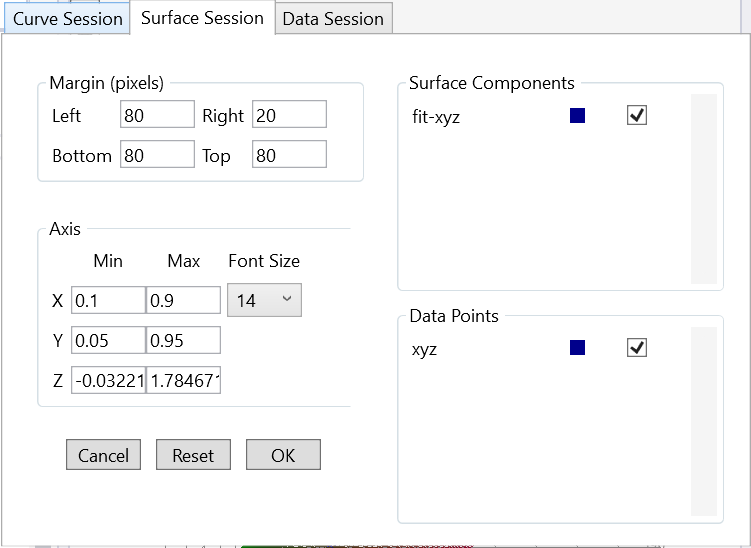
Clicking on the “Plot Settings” button opens up the session management tab illustrated in figure 4. Users can customize the display using the following UI controls at the left of GDE “Surface Session” tab.

•

Margin, set the display margin in the unit of pixels around the plotting area.
•

Axis $x$ min/max, set the $x$ axis range in 3-d display.
•

Axis $y$ min/max, set the $y$ axis range in 3-d display.
•

Axis $z$ min/max, set the $z$ axis range in 3-d display.
•

Font size, set the text font size on the 3-d plot.
•

Cancel, cancel the setting change.
•

Reset, reset the settings back to default values.
•

OK, plot the surface session using the current customized settings.

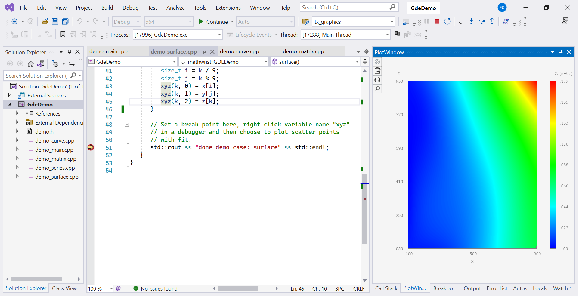
The right of the “Surface Session” tab lists all surface components and 3-d scatter points. In this code example Listing 1, note that prefix “fit-” is added to variable name xyz in the list of surface components and matrix object xyz appears as a scatter point component in figure 4(a).

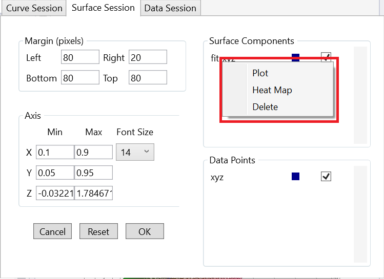
In GDE “Surface Session”, we can plot only one surface component but multiple scatter point components in the same display each time the OK button is clicked. Clicking the checkbox to include a surface component will automatically exclude all other surface components. Alternatively, users can directly right click the name of a surface component. A context menum will popup as illustrated with the red box area in figure 4(b). The “Plot” context menu command will render this surface component in 3-d display. The “Heat Map” command plots this surface component as a heat map as illustrated in Figure 5. The “Delete” command will remove the component from the surface session.

The data point section has 3 columns, component name, code coding and a checkbox respectively. Users can check multiple data point components to plot them together. Uncheck a scatter point component will automatically exclude its surface fit from the plot. Right click a scatter point component name, the context menu has only “Delete” command to delete this point component and its surface fit (if any) from the session.

5 NPL Plottable Types

The following NPL C++ classes are recognized as 3-d plottables and can be added to GDE surface session for plotting.

•

mathwrist::FunctPiecewise2DConst, a piecewise constant function.
•

mathwrist::BilinearSurface, a bilinear surface.
•

mathwrist::BSplineSurface, a B-spline surface.
•

mathwrist::ChebyshevSurface, a Chebyshev surface.
•

mathwrist::Matrix, mathwrist::Matrix::View and mathwrist::Matrix::ViewConst, a matrix or a direct matrix view that has 3 rows or 3-columns.

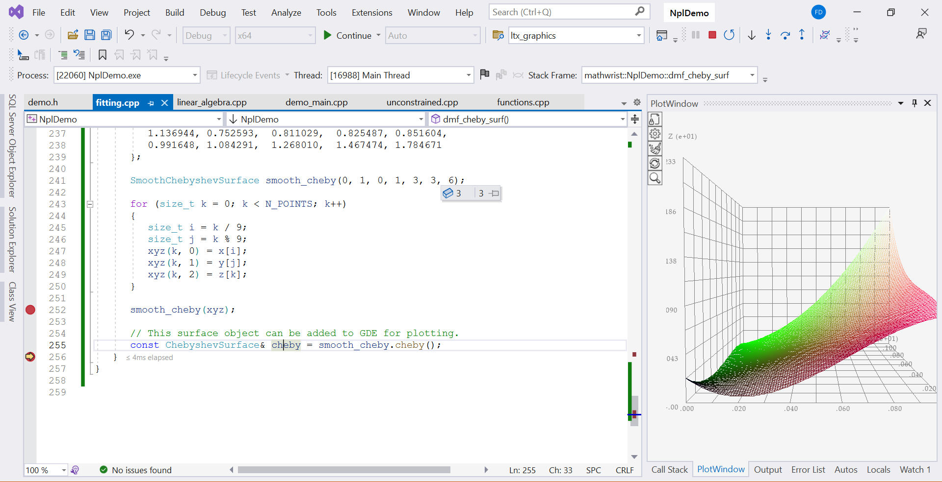
Figure 6 is an example screen shot of plotting a NPL surface object in GDE. This example is largely same as code Listing 1 except that we are now fitting the xyz scatter points to a smooth mathwrist::ChebyshevSurface object. Right click the variable name cheby of the surface object in Visual Studio debug session, and then click “plot cheby” from debugging context menu. GDE then renders the surface display in GDE plot window at the right side of the IDE.

GDE Surface Plots Mathwrist User Guide Series