GDE Overview
Mathwrist User Guide Series

(October 13, 2023)

Abstract

This document gives a high level overview of using Mathwrist’s Graphical Debugging Extension (GDE) tool for scientific visualization in Microsoft Visual Studio IDE while developing C++ numerical programs. More detailed information can be found in subsequent user guide series by feature chapters.

1 Introduction

Mathwrist’s Graphical Debugging Extension (GDE) product is a C++ debugging extension tool for Microsoft Visual Studio 2022 community, professional and enterprise editions. It allows scientists and engineers to directly view data and math objects while performing C++ numerical programming or prototyping tasks. By rendering scientific plots inside the Visual Studio IDE, users can obtain immediate visual feedback along the course of developing and refining their algorithms or mathematical models.

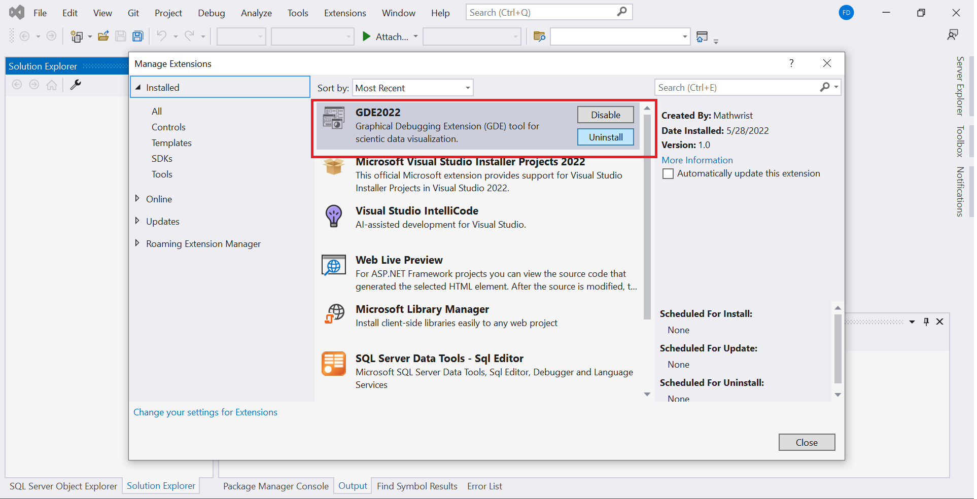
GDE is published to Visual Studio Extension Marketplace. Users can download the software from the marketplace, or directly install it under Visual Studio menu Extensions $|$ Manage Extensions and search for “GDE” from the list of online extensions. Once installed to Visual Studio as illustrated in Figure 1, GDE can be used free of charge with limited features. In order to run GDE of full features, a valid license file is required.

Figure 1: GDE Installed in Visual Studio

Mathwrist uses a standard Windows software installer to deploy a license activation application and its C++ numerical programming library (NPL) product to user’s desktop. GDE and NPL use the same license activation application to generate a node-locked license file. This software installer will be available for download from Mathwrist website Pricing $|$ Free $|$ Get started under either NPL or GDE product. After a purchase order is completed on Mathwrist website, the installer link will also be available from user’s order history page. Please refer to NPL user guide for the details of license activation.

2 Plottable Data Types

By default, C++ native double static array and std::vector $<$ double $>$ are automatically supported for plotting as “vector” data. This is a free feature to all users. Full featured software licenses will allow users to import user-defined “vector” and “matrix” C++ data types to GDE via a plottable specification json file. Most importantly, many built-in block data types defined in Mathwrist’s C++ Numerical Programming Library (NPL) are registered in GDE as plottables. NPL users have the advantage of working in an integrated environment equipped with numerical algorithms and visualization tools.

Let $x$ be the variable name of a plottable object in a C++ debugging program. By right clicking the variable name $x$ at a break point where object $x$ is in scope, GDE dynamically adds a “plot $x$ ” command to Visual Studio debugging context menu. Clicking this context menu command will either directly display object $x$ in a GDE plot window or allow users to choose relevant plotting format from a popup window. Users can further customize the display settings of the plot window and manage plottable objects in various plot sessions.

3 Plot Window

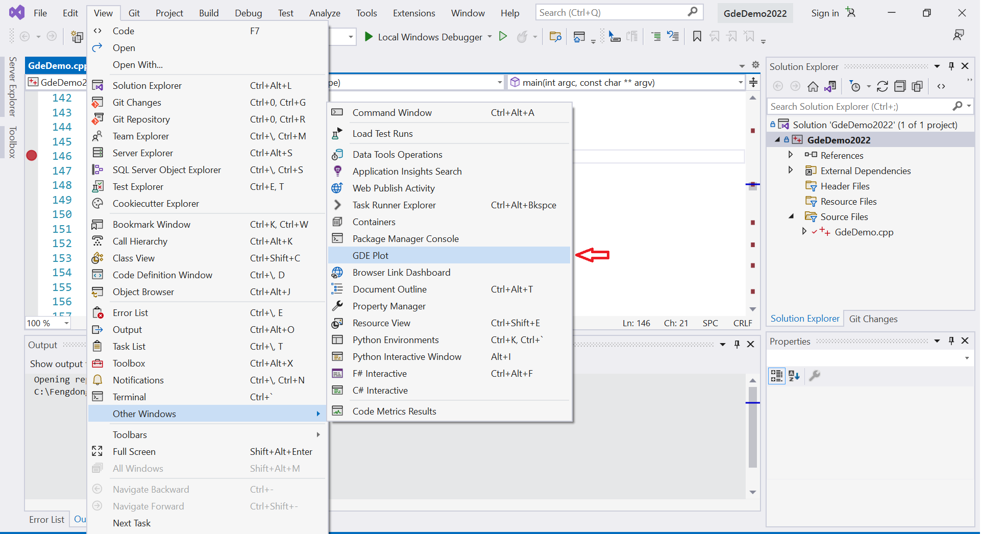
After a successful installation of the GDE package, GDE will register a menu item to Visual Studio IDE, under the path Views $|$ Other Windows $|$ GDE Plot. This is illustrated by the red arrow in figure 2. Clicking this menu item will bring up the GDE plot window to the front of IDE.

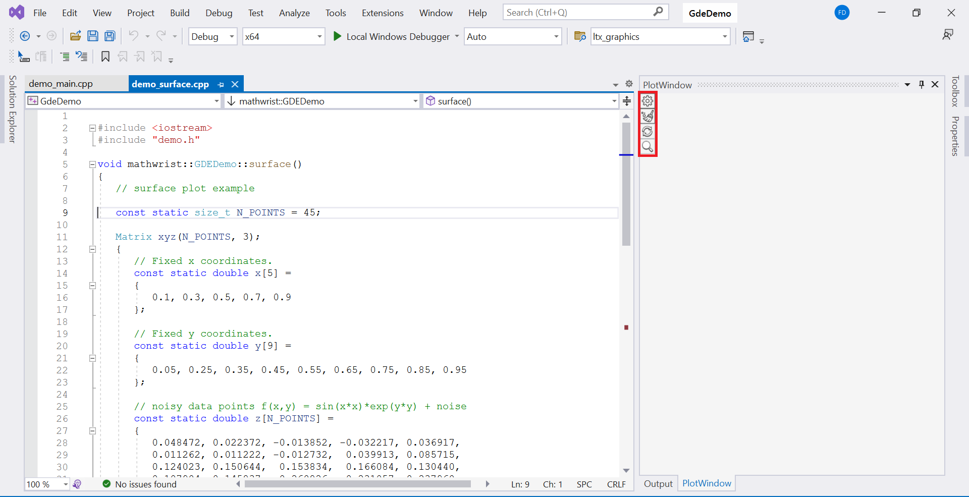
Like other Visual Studio tool windows, GDE plot window can be docked within the standard IDE layout panel, or can be undocked as a floating window at a convenient location on the screen. In the demo example of figure 3, we have docked the GDE plot window side by side to the source code editor, tabbed together with other Visual Studio debugging windows, i.e. callstack, output windows.

Figure 3: Plot and Source Code Side by Side

4 Settings

The red rectangle area in figure 3 is a group of GDE control buttons, , , and from top to bottom respectively. Moving the mouse over these buttons, we can see a tool tip text block emerging to indicate the purpose of these buttons, “Documentation”, “Plot Settings”, “Clear Plot” and “3-d Zooming”. Initially, “3-d Zooming” button is disabled in gray color. When a 3-d plottable object is displayed in the plot window, this button will then be enabled to support zooming 3-d objects.

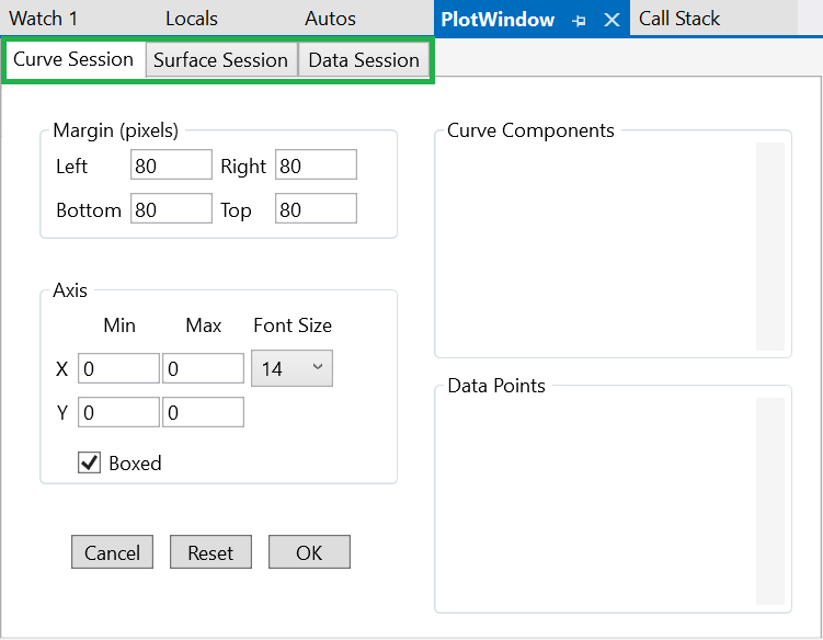
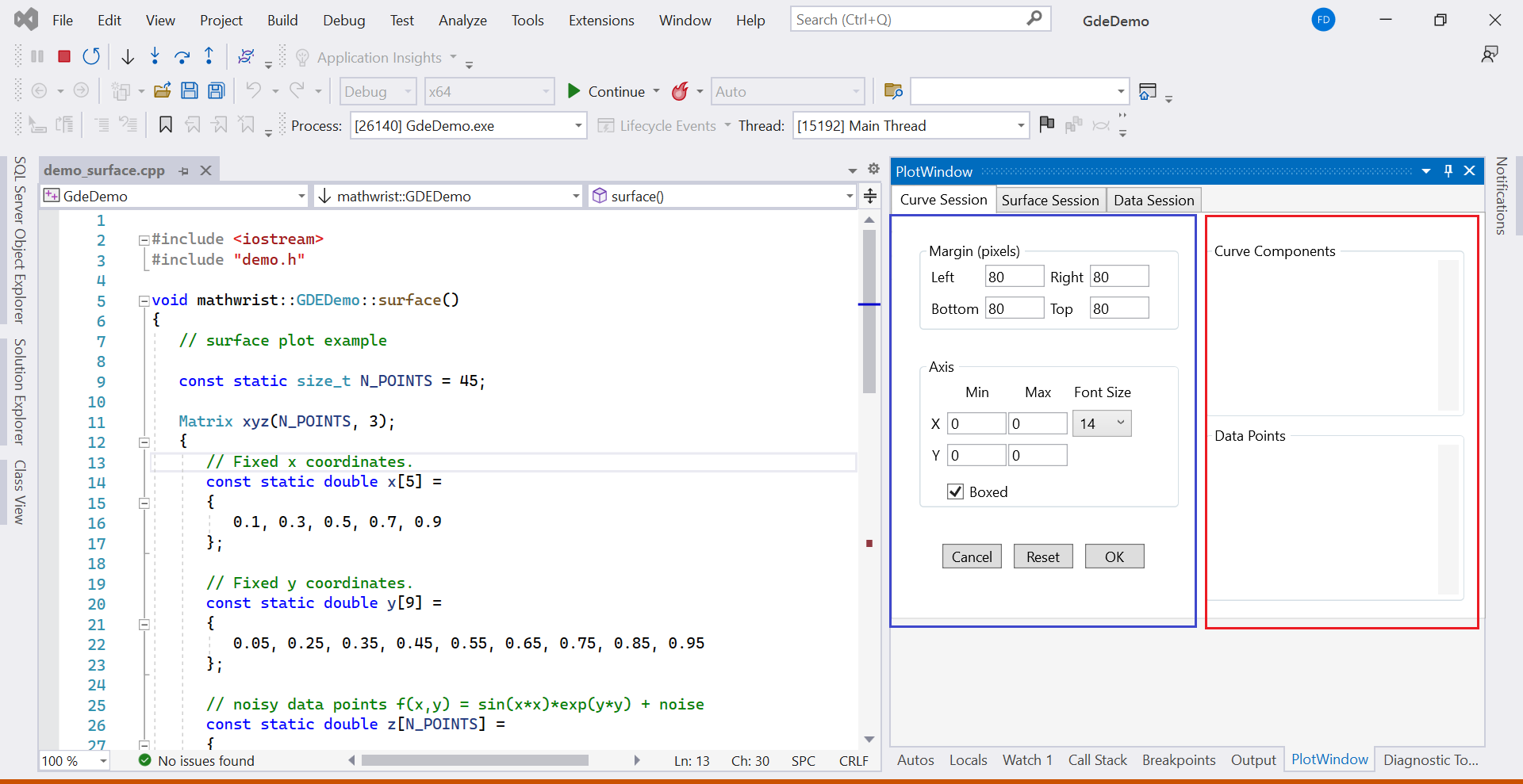
The “Plot Settings” button is used to customize display control parameters. It opens up a plot settings window illustrated in example figure 4. This settings window has 3 tabs “Curve Session”, ”Surface Session” and “Data Session” marked by a green rectangle in figure 4. Each tab allows users to set display control parameters and manage plottable components in the corresponding session.

When a plottable object is sent to the plot window for display, depending on the nature of this object, it will be cached in one of these three sessions. We shall call the session that is currently displayed in the plot window the “Active Session”. When the “Clear Plot” button is clicked, the display window and all components of the active session are cleared.

5 Object Bookkeeping

Plottable objects are bookkept by their unique names in each session. Within the same session, if two objects with the same variable name $x$ are added, the latter one always replaces the first object. In other words, one session only caches a unique name $x$ in its plottable component list.

What could be interesting to users is that, if the debuggee program stops at a break point where an object of name $x$ is in scope in the current debugging call stack, further if this object has the same data type as the plottable component represented by variable $x$ in the active session, then this plottable component will be automatically updated by object $x$ in the current stack. This feature could be very useful when we want to visualize how $x$ evolves, i.e. over iterations.

It is important to keep in wind that at each break point, the plottable name $x$ always represents the current live object in the current debugging call stack. All plottable components in a session are cached until they are explicitly deleted by the user. They are automatically updated when i) the debuggee stops at a breakpoint; and ii) their names and types match the live objects in the current call stack. When the debuggee process terminates, all plottable objects are still saved in relevant GDE sessions.

6 Session Management

As discussed earlier, clicking the “Plot Settings” button opens up a plot settings window that has “Curve”, “Surface” and “Data” three session management tabs. A full picture of this plot setting window within Visual Studio IDE is illustrated in figure 5. The left part of each tab, marked in a blue box area, contains controls that allow users to customize the display of that session. The right part of the tab, marked in a red box, contains a list of plottable components that have been added to the session. Right clicking a component name will trigger a context menu that allows users to delete this component from the current session, or display the component in applicable alternative plot types. We will discuss more session-specific details in subsequent GDE user guide series.

7 Plottable Specification File

By default, std::vector $<$ double $>$ and C++ native static array, i.e. double x[100], are recognized by GDE as vector plottables. Users may have their own implementation of vectors and matrices. It is possible to register user defined data types to GDE via a specification json file.

Each time when GDE is loaded to Visual Studio, it searches for a json file “mathwrist.gde.spec.json” under the Windows user profile directory. This directory has environment variable name “USERPROFILE” in Windows 10 and 11, which points to “C: $\backslash$ Users $\backslash$ xxx” directory where “xxx” is the user name. If the plottable specification file is found present in the user profile directory, GDE will import these user defined data types as plottable types.

7.1 Vector Types

In this section and the next “Matrix Types” section, we will illustrate how to specify a user-defined data type by examples. First, please find the following C++ code Listing 1 from the demo.h header file in the “GdeDemo” project that we shipped together with GDE installation.

Listing 1: C++ Buffer Class

1 namespace mathwrist

2 {

3 class GDEDemo

4 {

5 public:

6 // Demo a user defined data buffer type to be plotted in GDE.

7 // Demo: plot objects of user defined data types in in Visual

8 // Studio debug session. Please copy "mathwrist.gde.spec.json"

9 // file to your Windows user profile directory, C:\Users\xxx,

10 // where xxx is your Windows user name. Please also read GDE

11 // documentation series for details.

12 class Buffer

13 {

14 double* m_data;

15 size_t m_size;

17 // Disable copy c-tor and assignment for simplicity of demo.

18 Buffer(const Buffer&) = delete;

19 const Buffer& operator= (const Buffer&) = delete;

21 public:

22 explicit Buffer(size_t n = 0) : m_data(0), m_size(n)

23 {

24 if (n > 0)

25 m_data = new double[n];

26 }

27 ~Buffer() { delete[] m_data; }

29 size_t size() const { return m_size; }

31 double operator[](size_t i) const

32 {

33 if (i >= m_size)

34 throw "Index out of buffer size.";

36 return m_data[i];

37 }

39 double& operator[](size_t i)

40 {

41 if (i >= m_size)

42 throw "Index out of buffer size.";

44 return m_data[i];

45 }

46 };

This simple buffer class stores dynamically allocated memory to its class member m_data and the number of elements to member m_size. The corresponding json specification of this buffer class starts from line 3 to line 7 in code Listing 2. Keyword “Vectors” at line 2 tells GDE that this specification block contains a list of vector types. Each open/close bracket {…} in between [ and ] is a single vector-type specification.

The keyword “TypeName” at line 4 indicates that the exported vector type is called mathwrist::GDEDemo::Buffer. Note that namespace “mathwrist” and outer class name “GDEDemo” are all required in order to correctly refer to the given type. Keyword “MemberSize” at line 5 indicates the vector size is stored in class/struct data member m_size. And finally keyword “MemberPointer” at line 6 indicates the vector data storage pointer is m_data.

Alternatively, a vector type specification can provide the class/struct member name of the one-beyond-last element instead of specifying the vector size. This is illustrated from line 8 to line 12 for std::vector $<$ double $>$ . Here, “MemberPointer” is still the starting memory address of the std vector, which is _Mypair._Myval2._Myfirst in Microsoft’s std::vector implementation. Keyword “MemberLast” indicates that the memory address of the one-beyond-last element can be obtained from class/struct data member _Mypair._Myval2._Mylast.

Listing 2: Vector Plottable Specification

2 "Vectors": [

3 {

4 "TypeName": "mathwrist::GDEDemo::Buffer",

5 "MemberSize": "m_size",

6 "MemberPointer": "m_data"

7 },

8 {

9 "TypeName": "std::vector<double,std::allocator<double>>",

10 "MemberPointer": "_Mypair._Myval2._Myfirst",

11 "MemberLast": "_Mypair._Myval2._Mylast"

12 }

13 ],

7.2 Matrix Types

In the same demo.h header file, we also provided a C++ matrix class definition that uses std::vector as data storage. The complete code example is included in Listing 3. Its json specification is given in Listing 4.

Listing 3: C++ Matrix Class

1 // Demo a user defined matrix type to be plotted in GDE.

2 class Matrix

3 {

4 size_t m_rows;

5 size_t m_cols;

6 bool m_row_wise;

7 std::vector<double> m_storage;

9 public:

10 Matrix(size_t m, size_t n, bool row_wise = true) :

11 m_rows(m), m_cols(n), m_row_wise(row_wise), m_storage(m * n) {}

13 size_t n_rows() const { return m_rows; }

14 size_t n_cols() const { return m_cols; }

16 double operator()(size_t i, size_t j) const

17 {

18 if (i >= m_rows || j >= m_cols)

19 throw "Index out of buffer size.";

21 return m_storage[m_row_wise ? i * m_cols + j : j * m_rows + i];

22 }

24 double& operator()(size_t i, size_t j)

25 {

26 if (i >= m_rows || j >= m_cols)

27 throw "Index out of buffer size.";

29 return m_storage[m_row_wise ? i * m_cols + j : j * m_rows + i];

30 }

31 };

Listing 4: Matrix Plottable Specification

1 "ConsecutiveMatrices": [

2 {

3 "TypeName": "mathwrist::GDEDemo::Matrix",

4 "MemberRowSize": "m_rows",

5 "MemberColumnSize": "m_cols",

6 "MemberPointer": "m_storage._Mypair._Myval2._Myfirst",

7 "RowMajor": "m_row_wise"

8 }

9 ],

Here, keyword “ConsecutiveMatrices” tells GDE that this specification block is to export matrix types that use consecutive memory storage. We have only one type in this block, which is mathwrist::GDEDemo::Matrix following the keyword “TypeName” at line 3.

Line 4 and 5 indicate the number of rows and columns are stored in class/struct data member m_rows and m_cols, after keywords “MemberRowSize” and “MemberColumnSize” respectively. At line 6, keyword “MemberPointer” tells GDE that the memory address of matrix element storage can be obtained by following the chain of data members m_storage._Mypair._Myval2._Myfirst.

Lastly, keyword “RowMajor” at line 7 is used to specify whether the matrix uses row-major or column-major memory storage. In this example, we tell GDE the row-major flag is stored in class/struct member m_row_wise. If this line is missing, by default we interpret the matrix uses row-major storage. Alternatively, users can specify key-value pairs “RowMajor”: “TRUE” or “RowMajor”: “FALSE” for matrix types that consistently use row-major or column-major storage.

GDE Overview Mathwrist User Guide Series