GDE Data Plots
Mathwrist User Guide Series

(January 20, 2023)

Abstract

This document is a user guide of using Mathwrist’s Graphical Debugging Extension (GDE) tool to visualize raw data in Microsoft Visual Studio IDE when debugging a C++ program. For an overview of GDE, please refer to our “GDE Overview” user guide.

1 Introduction

In this document, we focus on GDE “Data Session” and give details on how to use GDE to plot raw data of C++ standard types, Mathwrist’s Numerical Programming Library (NPL) data types and user specified plottable types that are defined in a json file. It is highly recommended to first read our “GDE Overview” user guide to have a high level understanding of GDE. The details of how to export user defined data types to GDE via a json specification file are covered in our “GDE Overview” user guide as well.

In general, we treat raw data plottables as either vectors or matrices. Vector data includes C++ static array, std::vector $<$ double $>$ , user defined vector data types, and 1-row or 1-column matrices. Objects of vector data type can be plotted as data series or histograms. Multi-row and multi-column matrix objects can be plotted as row data series, column data series, histogram and heat map. Users have opportunities to choose the plot format in relevant contexts.

2 Walkthrough Example

All code examples listed here are part of the “GdeDemo” Visual Studio project that is shipped together with GDE installation.

2.1 Vector Objects

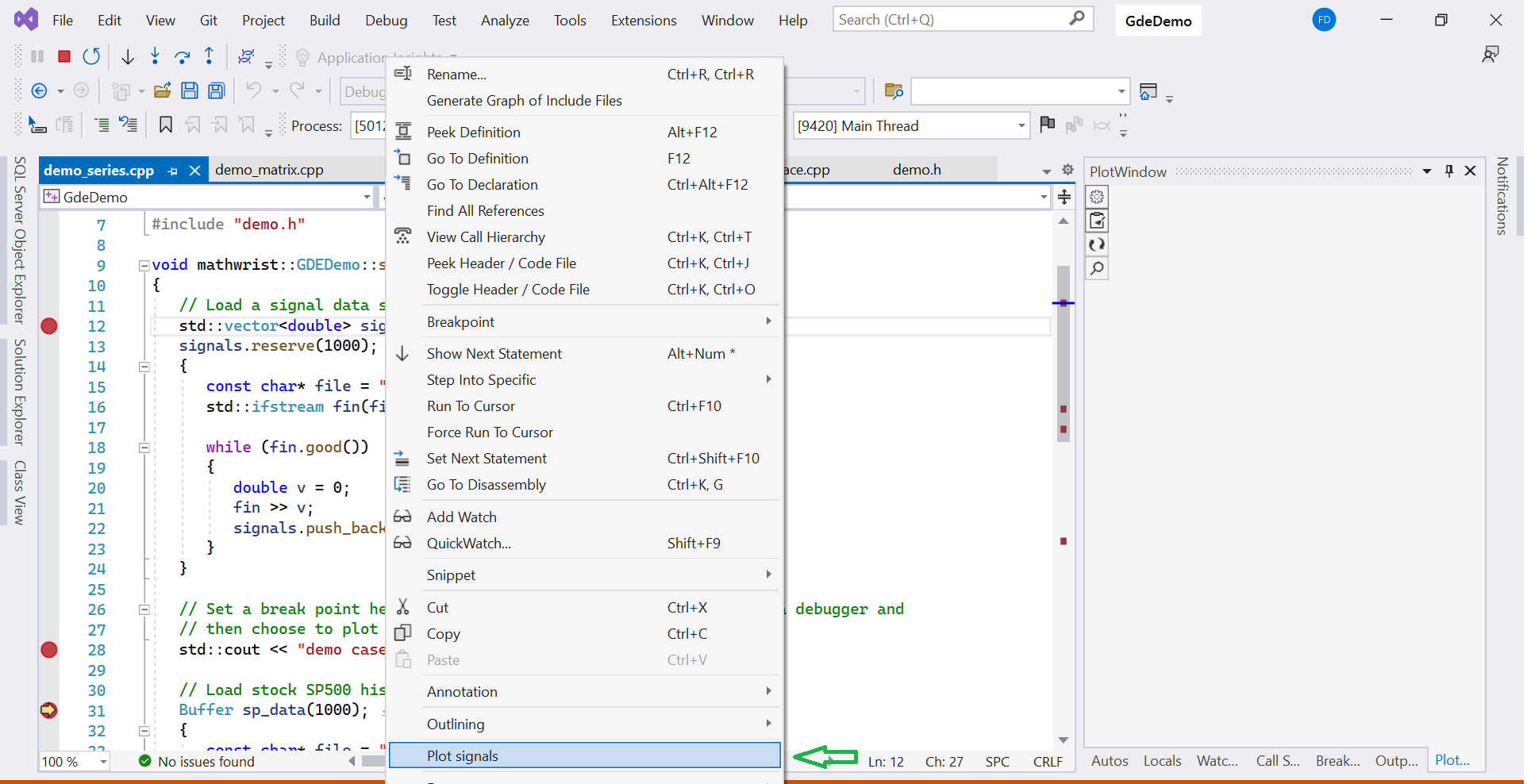
The sample code Listing 1 demonstrates plotting vector data as series and histograms. To run this example, we set command line argument –series in debugging property of “GdeDemo” project. First, from line 11 to line 22, we read a series of signal data from a text file and store it in the standard std::vector variable signals. Since std::vector $<$ double $>$ is a standard type supported by GDE internally, variable signals is recognized as a built-in plottable data type. The sequence of steps to display this raw data object signals is the following:

1.

When the debuggee process stops at a breakpoint line 27, right clicking the variable name signals brings the debugging context menu to the front of IDE in Figure 1.
2.

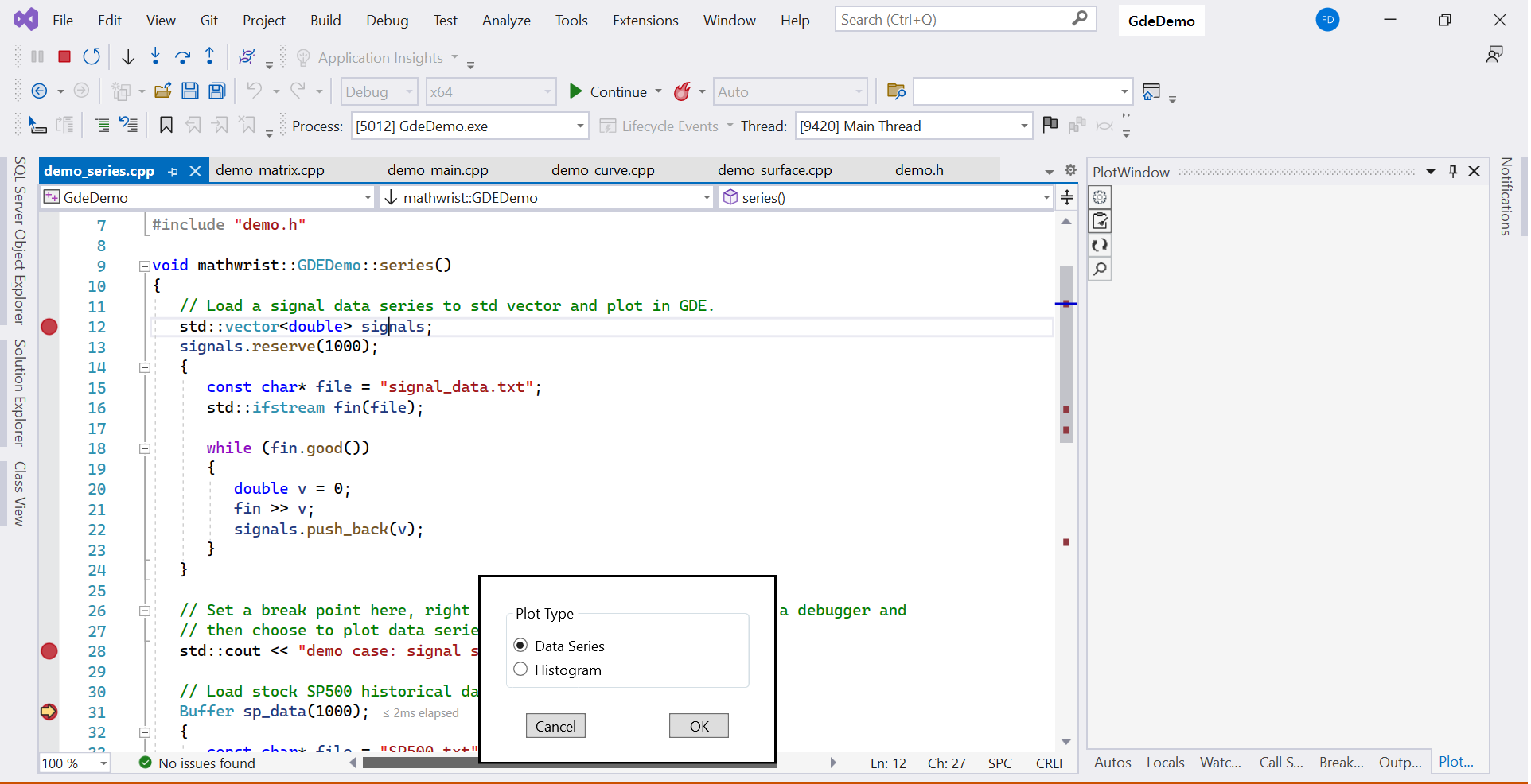
Click the “Plot signals” command from the context menu triggers a data plot choice popup window in Figure 2. This popup allows users to choose either data series plot or histogram plot.
3.

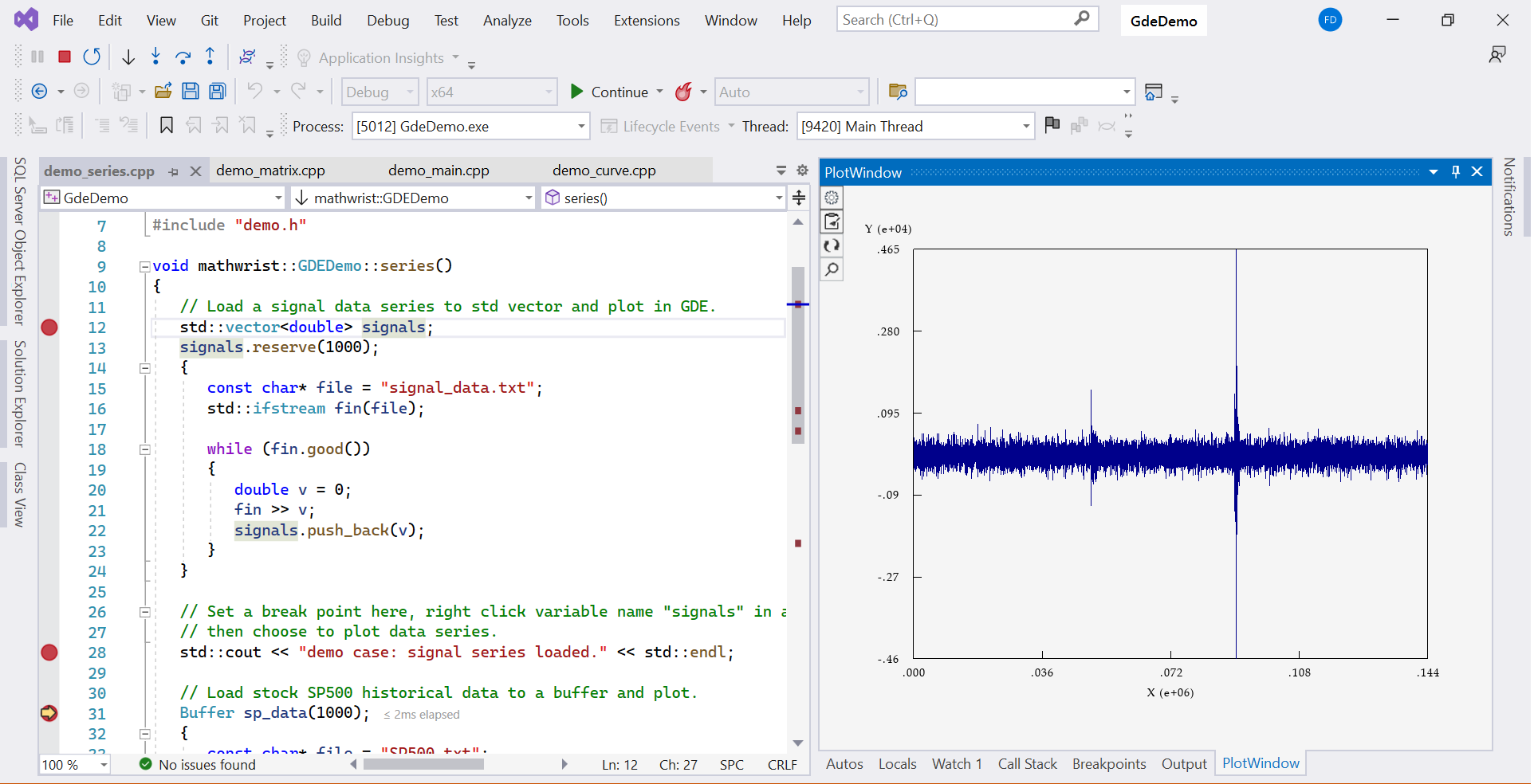
Check the “Data Series” radio button and click OK in the popup window. The data series plot is displayed in the plot window in Figure 3.

Listing 1: Vector Plot Example

1 #include <algorithm>

2 #include <iostream>

3 #include <fstream>

4 #include <vector>

6 #include "demo.h"

8 void mathwrist::GDEDemo::series()

9 {

10 // Load a signal data series to std vector and plot in GDE.

11 std::vector<double> signals;

12 signals.reserve(1000);

13 {

14 const char* file = "signal_data.txt";

15 std::ifstream fin(file);

17 while (fin.good())

18 {

19 double v = 0;

20 fin >> v;

21 signals.push_back(v);

22 }

23 }

25 // Set a break point here, right click variable name "signals" in a

26 // debugger and then choose to plot data series.

27 std::cout << "demo case: signal series loaded." << std::endl;

29 // Load stock SP500 historical data to a buffer and plot.

30 Buffer sp_data(1001);

31 {

32 const char* file = "SP500.txt";

33 std::ifstream fin(file);

35 for (int i = 0; i < 1001 && fin.good(); ++i)

36 {

37 fin >> sp_data[i];

38 }

39 }

41 // Copy stock SP500 data to a native array and plot.

42 Matrix sp_returns(1000,1);

43 for (int i = 0; i < 1000; ++i)

44 {

45 sp_returns(i,0) = std::log(sp_data[i+1] / sp_data[i]);

46 }

48 // Set a break point here, right click variable name "sp_data"

49 // or "sp_array" in a debugger and then choose to plot data

50 // series.

51 std::cout << "done demo case: data_series" << std::endl;

52 }

Next, from line 30 to 39, we read stock market SP500 index historical data from a text file and store it to a user-defined Buffer data structure with variable name sp_data. As we discussed in “GDE Overview” user guide, by supplying a “mathwrist.gde.spec.json” plottable specification json file and exporting user-defined type Buffer to GDE, variable sp_data at line 31 is also recognized as a plottable object. At breakpoint point line 43, one can repeat the same steps as we plot signals except that now the context menu item becomes to “Plot sp_returns”.

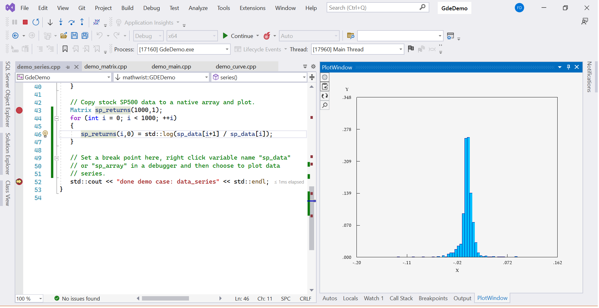
Lastly, we compute the daily log return of SP500 data and store it to user-defined Matrix type with variable sp_returns from line 43 to 46. Matrix is also exported to GDE through the specification json file. Note that matrix object sp_return has only 1 column, hence is treated as a vector. Right clicking variable name sp_returns when the debugger stops at break point line 51, we can choose “Plot sp_return” as a histogram plot as illustrated in Figure 4.

2.2 Matrix Objects

Sample code Listing 2 illustrates a multi-row and multi-column matrix object can be plotted as data series, histograms and heat maps. This example requires to set command line argument –matrix to “GdeDemo” project.

Listing 2: Matrix Plot Example

2 #include <iostream>

3 #include <random>

4 #include "demo.h"

6 void mathwrist::GDEDemo::matrix()

7 {

8 const size_t n_x_points = 201;

9 const size_t n_y_points = 201;

11 // Populate a standard 2-d Gaussian distribution

12 Matrix z(n_x_points, n_y_points);

13 {

14 const double dx = 4.0 / (n_x_points - 1);

15 const double dy = 4.0 / (n_y_points - 1);

17 for (size_t i = 0; i < n_x_points; ++i)

18 {

19 double x = -2 + i * dx;

20 for (size_t j = 0; j < n_y_points; ++j)

21 {

22 double y = -2 + j * dy;

23 z(i,j) = 0.5 / std::_Pi * std::exp(-0.5 * (x * x + y * y));

24 }

25 }

26 }

28 // Set a break point here, right click matrix variable name "z"

29 // in a debugger and then choose to plot the Gaussian density

30 // as a heat map.

31 std::cout << "demo case: gaussian density heat map" << std::endl;

33 // Populate a 5 x 6 matrix but in column-wise storage major.

34 Matrix G(5, 6, false);

35 for (int i = 0; i < 5; ++i)

36 {

37 for (int j = 0; j < 6; ++j)

38 G(i, j) = j;

39 }

41 // Set a break point here, right click matrix variable name "G"

42 // in a debugger and then choose to plot heat map to see the

43 // color coding.

44 std::cout << "done demo case: matrix" << std::endl;

46 }

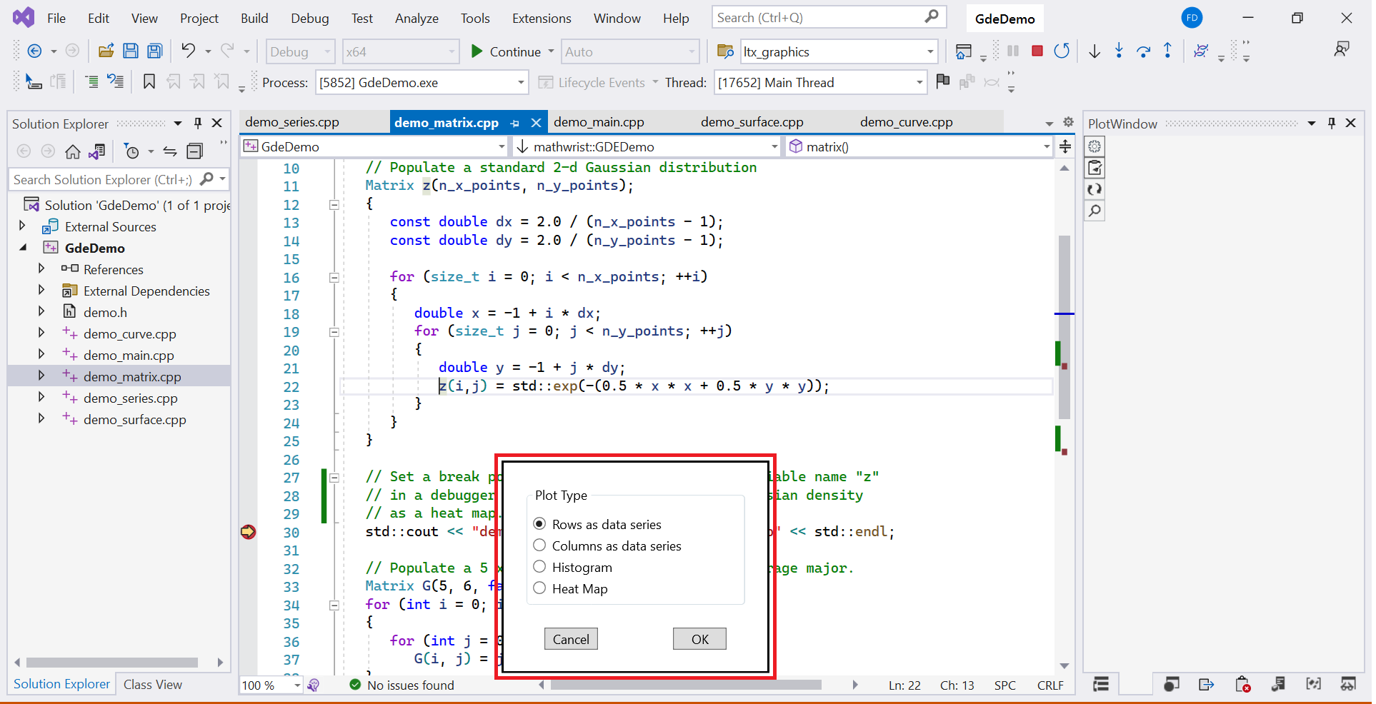
Between line 11 and 25, we populate a $101\times 101$ square matrix $z$ with standard Gaussian density. When the demo debug program stops at break point line 30, right clicking on variable name $z$ and choose “Plot $z$ ” from Visual Studio debugging context menu. A popup window Figure 5 provides choices to plot the rows or columns of matrix $z$ as data series, or alternatively plot all elements to a histogram or a heat map.

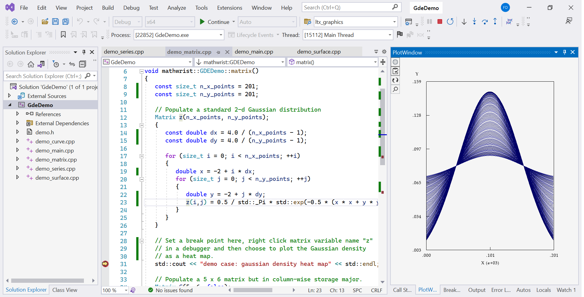
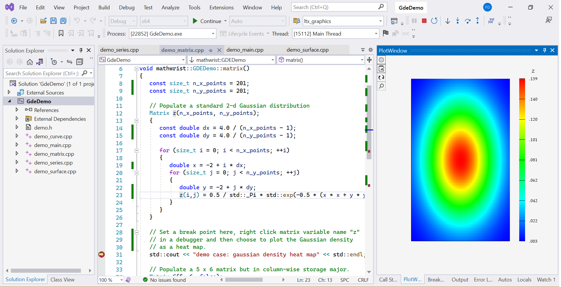
Since $z$ is a symmetric matrix, plotting row series or column series does not matter in this example. But in general, this display orientation choice is remembered in GDE’s data session. Figure 6 illustrates the data series plot of matrix $z$ . Figure 7 is the final display of plotting matrix $z$ in heat map format.

3 Session Management

After we plot signals and sp_returns in example Listing 1, these two vector type objects are added to the “Arrays/Vectors” section of GDE data session. We can start the demo program again with command line argument –matrix and plot matrix object $z$ , which is added to the “Matrices” section on GDE data session. Clicking the “Plot Settings” button , we can see the “Data Session” tab illustrated by Figure 8.

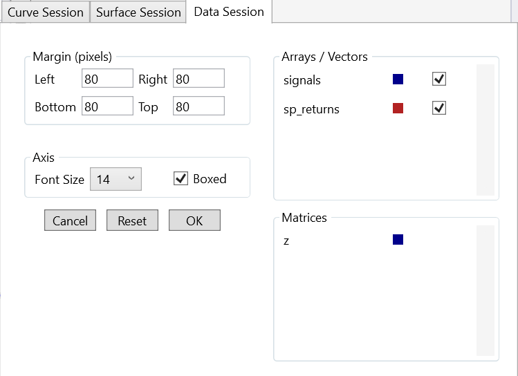
Users can then customize the display using the following UI controls at the left of the tab.

•

Margin, set the display margin in the unit of pixels around the plotting area.
•

Font size, set the text font size on the data plot.
•

Boxed, if selected, the plot area will display a solid line at each border.
•

Canel, cancel the display setting change.
•

Reset, reset the settings back to default values.
•

OK, plot the data session using the current customized settings.

On the right side of the data session tab, the top “Arrays/Vectors” section lists array/vector like plottable components. The bottom part lists matrix plottable components. In this example, we see the buffer object signals is recognized as “array/vector” type. One-column matrix object sp_return is treated as a vector and appears in “Arrays/Vectors” section as well. Matrix object $z$ on the other hand appears in the bottom section.

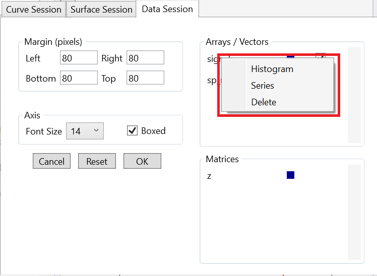
The “Arrays/Vectors” section has three columns, variable name, color coding and a checkbox. Right click on a variable name, a context menu appears as the red box area in Figure 9. Menu item “Histogram” and “Series” allow users to plot this component as a standalone histogram or data series. Menu item “Delete” will remove this component from the data session. The checkbox column is used to select multiple vector components and plot them together in the same data series display after clicking the OK button.

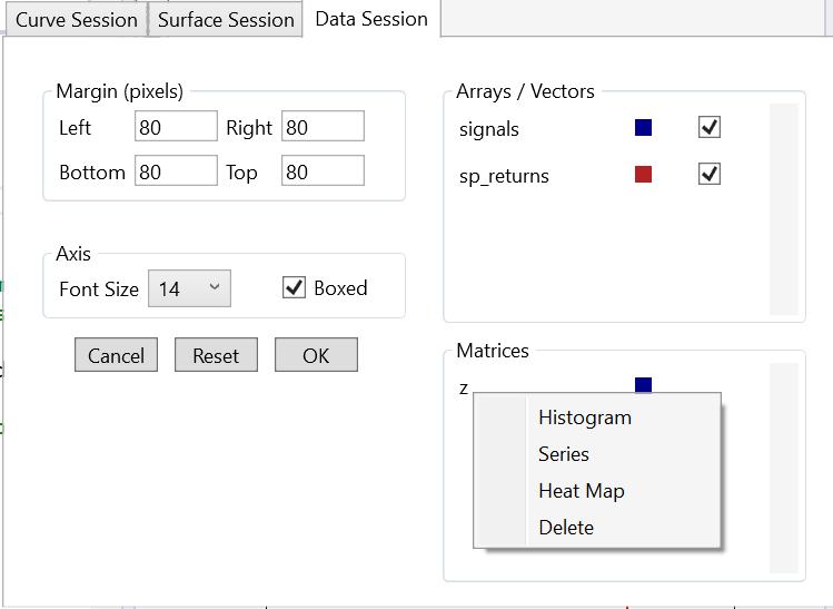
The “Matrices” section has only component name and color coding two columns, since matrix objects are always displayed separate from each other. Right click a component name brings up a context menu illustrated as the red box in Figure 10. Matrix objects can be plotted as histogram, series or heat map from the context menu. “Delete” command will remove a matrix plottable from the data session.

4 NPL Plottable Types

Mathwrist’s own buffer and matrix classes, mathwrist::ftl::Buffer $<$ double $>$ and mathwrist::Matrix, are treated the same way as user-defined vector and matrix plottable types. In addition, direct view objects from mathwrist::Matrix::View and mathwrist::Matrix::ViewConst classes are understood as matrix plottable as well. Here, a direct matrix view means that the view object directly mapps to some contiguous memory. Indirect matrix views, i.e. transposed view, matrix sub views, permutated views etc., are not supported as plottable types.

GDE Data Plots Mathwrist User Guide Series