GDE Dynamics Plots
Mathwrist User Guide Series

(January 20, 2023)

Abstract

This document is a user guide of using Mathwrist’s Graphical Debugging Extension (GDE) tool to visualize the dynamic process of certain numerical algorithms implemented in NPL. NPL is Mathwrist’s C++ numerical programming library. By visualizing how a mathematical problem is tackled numerically, scientists and engineers might be able to refine problem formulation, undstand model behavior or identify implementation issues easier.

1 Introduction

GDE dynamics display is designed to watch how certain quantities of interest evolve over time or iteratively make progress. NPL typically implements a numerical algorithm as a specific C++ solver class. Like all other NPL “plottable” types, a solver object that supports dynamics display is recognized by GDE at debugging time.

As usual, users can right click the variable name x of a solver object in Visual Studio debugger and then click context menu command “plot x” to triger the dyanmics display. However, a dynamics plottable object is not managed or stored by any of the GDE data, curve or surface sessions. Instead, it is a one-time animation, specific to the nature of the dynamics. Once the animation is complete, users can perform other visualization tasks as usual.

All NPL C++ classes that support GDE dynamics display have a public member function enable_watch(). Users need call this function in a C++ program to enable watching the dynamics. For the details of NPL, please refer to NPL white paper, API and code example documentation series. It is recommended to read through our “GDE Overview” user guide first to have a high level overview of GDE.

2 NPL Plottable Types

Root finding solver mathwrist::RootSolver1D and 1-d minimization solver mathwrist::MiniSolver1D are two dynamic plottables that users can watch how data points approach to the final solution along a smooth curve. This kind of dynamics plot effectively is a standard curve display with moving data points. It shares the same display control settings. i.e. margins, font size, etc., of the GDE curve session.

The second type of dynamics plot is to visualize multi-dimensional unconstrained optimization with the following solver classes.

•

mathwrist::LineSearchSteepestDescent
•

mathwrist::LineSearchNewton
•

mathwrist::LineSearchQuasiNewton
•

mathwrist::LineSearchConjugateGradient
•

mathwrist::TrustRegionExact
•

mathwrist::TrustRegionSteihaug

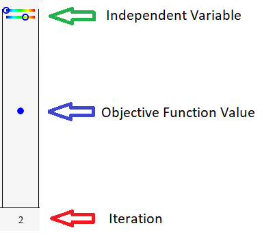
GDE displays optimization iterations as a sequence of frames. Users can watch the n-dimensional variable $x$ and objective function $f(x)$ change values across iteration frames. Figure 1 is such a frame example. $x$ and its numerical range are displayed at the top of the frame as small circles inside color gradient strips. If space accommodates, $n$ dimensional $x$ will display $n$ color gradient strips corresponding to $x_{i},i=0,\cdots,n-1$ starting from the top. Objective function value $f(x)$ is displayed as the blue dot in the middle of Figure 1. Its position along the $y$ axis indicates the value of $f(x)$ . Lastly, the iteration number is display at the bottom of the frame.

The third type of dynamics plottable includes the following constrained optimization solver classes. They also use a sequence of frames to represent optimization iterations. In general, linearly constrained optimization solvers have a phase-I feasibility stage and a subsequent optimality stage. In phase-I stage, the objective is to reduce constraint violation. GDE first uses red dots to represent the feasibility objective and switches back to blue dots in the optimality stage. If an independent variable $x_{i}$ has a lower/upper bound, GDE will in addition display a short vertical bar at the left/right end of the color gradient respectively.

•

mathwrist::GS_SimpleBoundNewton
•

mathwrist::GS_SimpleBoundQuasiNewton
•

mathwrist::GS_ActiveSetNewton
•

mathwrist::GS_ActiveSetQuasiNewton
•

mathwrist::Simplex
•

mathwrist::LP_ActiveSet
•

mathwrist::QP_ActiveSet
•

mathwrist::SQP_ActiveSet

Solving a nonlinear programming problem using the mathwrist::SQP_ActiveSet solver class involves major iterations and minor iterations. GDE dyanmics plot in this case will only display the original objective $f(x)$ in major iterations. Unlike linearly constrained optimization, $f(x)$ in SQP major iterations could be increasing or fluctuating. This is due to the nature that a SQP major iteration could be correcting the violation to nonlinear constraints at the cost of increasing $f(x)$ .

Lastly, the following model, curve and surface fitting solver classes are supported in GDE for dynamics display as well. However, please note that certain problem formulation has a closed-form solution and does not involve optimization iterations. In that situation, even though an object is of a legitimate solver type, GDE will not add a dynamics plot command to Visual Studio debugging context menu.

•

mathwrist::NLS_GaussNewton
•

mathwrist::NLS_Levenberg
•

mathwrist::NLS_General
•

mathwrist::SmoothBilinearSurface
•

mathwrist::SmoothChebyshevCurve
•

mathwrist::SmoothChebyshevSurface
•

mathwrist::SmoothSplineCurve
•

mathwrist::SmoothSplineSurface

3 Walkthrough Examples

3.1 Root Finding

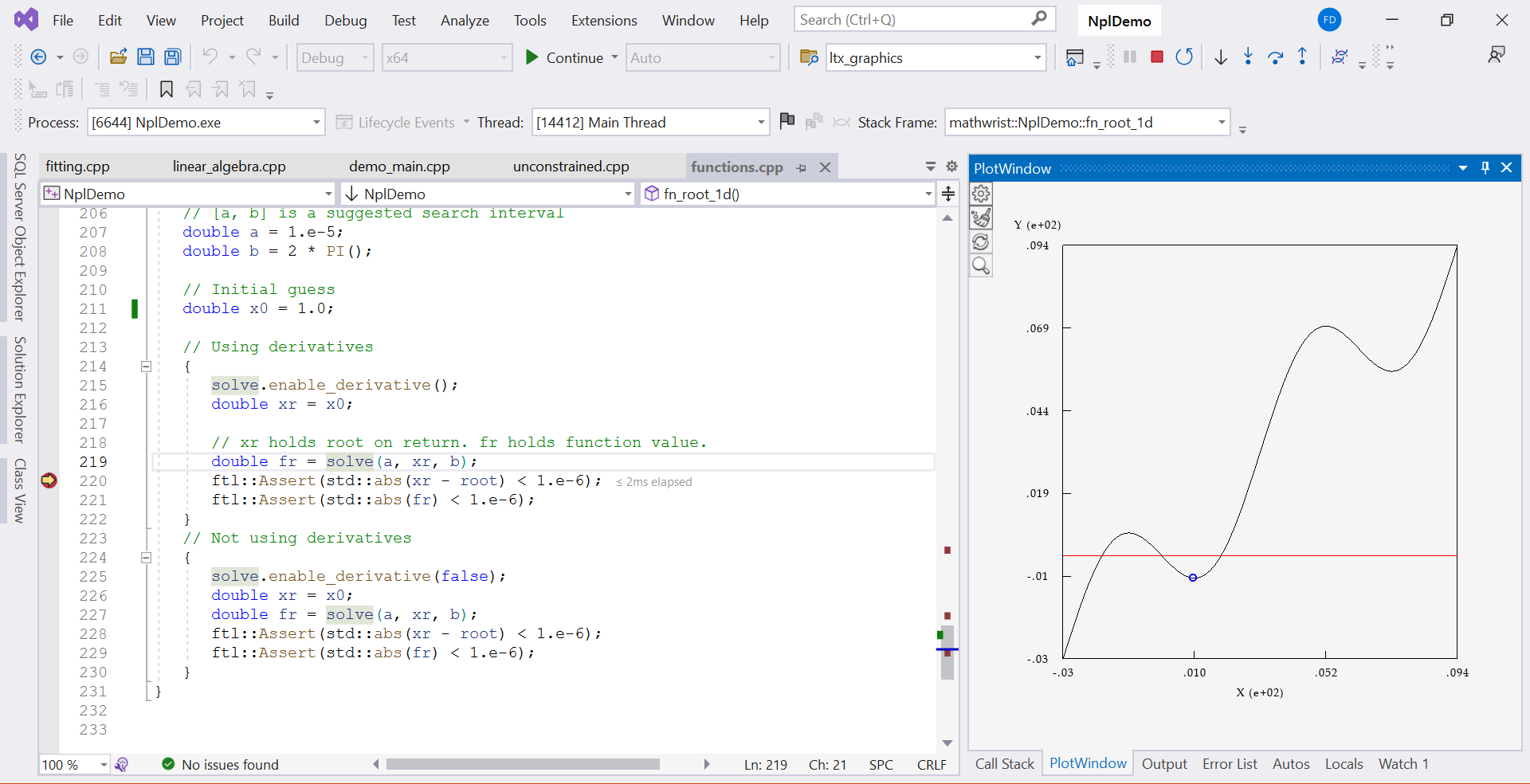
Code Listing 1 is a 1-d root-finding code example in the demo project that we shipped together with NPL installation. From line 3 to 14, an objective function Fx is defined locally. At line 16 and 17, we create an instance of Fx and pass it to the root finding solver. Note that at line 18, enable_watch() is called. This tells the solver to keep track of root finding iterations for dynamics display. After line 36 returns from the actual root-finding work, we set a break point at line 37.

Listing 1: Root Finding Plot Example

1 void NplDemo::fn_root_1d()

2 {

3 struct Fx : public Function1D

4 {

5 double eval(double x, double* _d1 = 0, double* _d2 = 0) const

6 {

7 if (_d1 != 0)

8 *_d1 = 1 - 2 * std::cos(x);

10 return x - 2 * std::sin(x);

11 }

12 // clone is not used, just provide a dummy implementation.

13 Function1D* clone() const { return 0; }

14 };

16 Fx f; // create the objective function

17 RootSolver1D solve(f); // create the solver object

18 solve.enable_watch();

20 // the root

21 double root = 1.895494;

23 // [a, b] is a suggested search interval

24 double a = 1.e-5;

25 double b = 2 * PI();

27 // Initial guess

28 double x0 = 1.0;

30 // Using derivatives

31 {

32 solve.enable_derivative();

33 double xr = x0;

35 // xr holds root on return. fr holds function value.

36 double fr = solve(a, xr, b);

37 ftl::Assert(std::abs(xr - root) < 1.e-6);

38 ftl::Assert(std::abs(fr) < 1.e-6);

39 }

40 // Not using derivatives

41 {

42 solve.enable_derivative(false);

43 double xr = x0;

44 double fr = solve(a, xr, b);

45 ftl::Assert(std::abs(xr - root) < 1.e-6);

46 ftl::Assert(std::abs(fr) < 1.e-6);

47 }

48 }

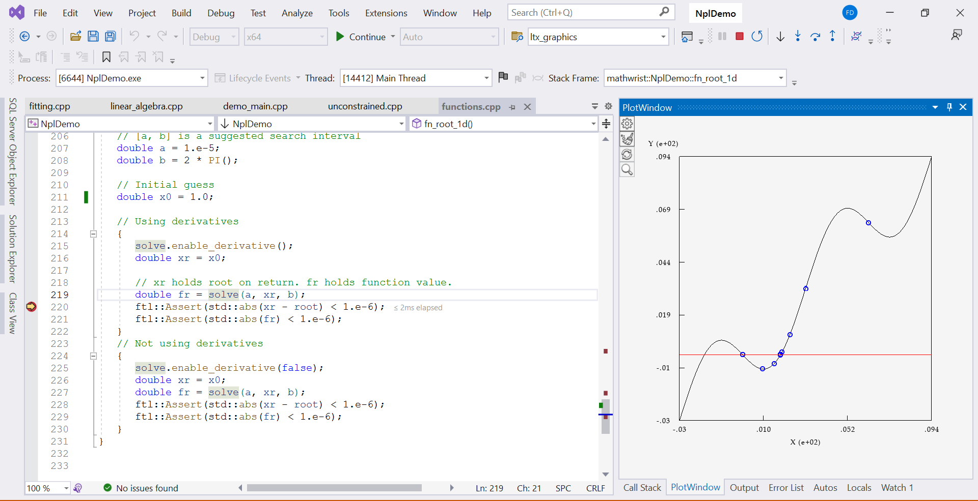
When the debuggee program stops at line 37, right click variable name solve and choose “plot solve” from the context menu. GDE plot window then starts to display an animation that plots the objective function as a smooth curve and a series of data points converging to the actual root. The start and end of this animation plot are illustrated in Figures 2 and 3.

3.2 Optimization

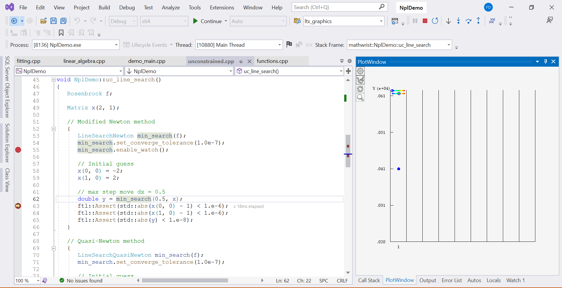
Code Listing 2 is an example in the same demo project that uses line-search methods to solve an unconstrained optimization problem. From line 2 to 32, an objective function Rosenbrock is defined. Line 36 creates an instance of the Rosenbrock objective function. Line 41 passes the objective function to the line-search solver object min_search.

Again, at line 43, we need call the enable_watch() function on the solver so that it saves necessary information for dynamics display. At line 50, the solver returns from the optimization work. We set a break point at line 51.

Listing 2: Optimization Example

1 // Rosenbrock’s function for unconstrained optimization example.

2 struct Rosenbrock : public FunctionND

3 {

4 // Clone is not used in the demo, just return a 0 pointer.

5 FunctionND* clone() const { return 0; }

7 double eval(const Matrix& x, Matrix* _g, Matrix* _H) const

8 {

9 double x1 = x(0, 0);

10 double x2 = x(1, 0);

11 const double retval = 100 * std::pow(x2 - x1 * x1, 2) +

12 std::pow(1 - x1, 2);

14 if (_g != 0)

15 {

16 (*_g)(0,0) = 400 * (x1 * x1 * x1 - x1 * x2) + 2 * x1 - 2;

17 (*_g)(1,0) = 200 * (x2 - x1 * x1);

18 }

20 if (_H != 0)

21 {

22 (*_H)(0, 0) = 1200 * x1 * x1 - 400 * x2 + 2;

23 (*_H)(0, 1) = -400 * x1;

24 (*_H)(1, 0) = -400 * x1;

25 (*_H)(1, 1) = 200;

26 }

28 return retval;

29 }

31 size_t dimension_size() const { return 2; }

32 };

34 void NplDemo::uc_line_search()

35 {

36 Rosenbrock f;

37 Matrix x(2, 1);

39 // Modified Newton method

40 {

41 LineSearchNewton min_search(f);

42 min_search.set_converge_tolerance(1.0e-7);

43 min_search.enable_watch();

45 // Initial guess

46 x(0, 0) = -2;

47 x(1, 0) = 2;

49 // max step move dx = 0.5

50 double y = min_search(0.5, x);

51 ftl::Assert(std::abs(x(0, 0) - 1) < 1.e-6);

52 ftl::Assert(std::abs(x(1, 0) - 1) < 1.e-6);

53 ftl::Assert(std::abs(y) < 1.e-8);

54 }

56 // Quasi-Newton method

57 {

58 LineSearchQuasiNewton min_search(f);

59 min_search.set_converge_tolerance(1.0e-7);

61 // Initial guess

62 x(0, 0) = 2;

63 x(1, 0) = -2;

65 // max step move dx = 0.5

66 double y = min_search(0.5, x);

67 ftl::Assert(std::abs(x(0, 0) - 1) < 1.e-6);

68 ftl::Assert(std::abs(x(1, 0) - 1) < 1.e-6);

69 ftl::Assert(std::abs(y) < 1.e-8);

70 }

71 }

When this debuggee program stops at line 51, right click on solver name min_search and choose “plot min_search” from context menu. GDE starts the dynamics animation in a series of frames in Figure 4. Each frame corresponds to an optimization iteration with the iteration numbers displayed along the $x$ axis at the bottom. The numerical scale of $f(x)$ is displayed vertically along the $y$ axis on the left of the dynamics plot. The end of the animation are shown in Figure 5.

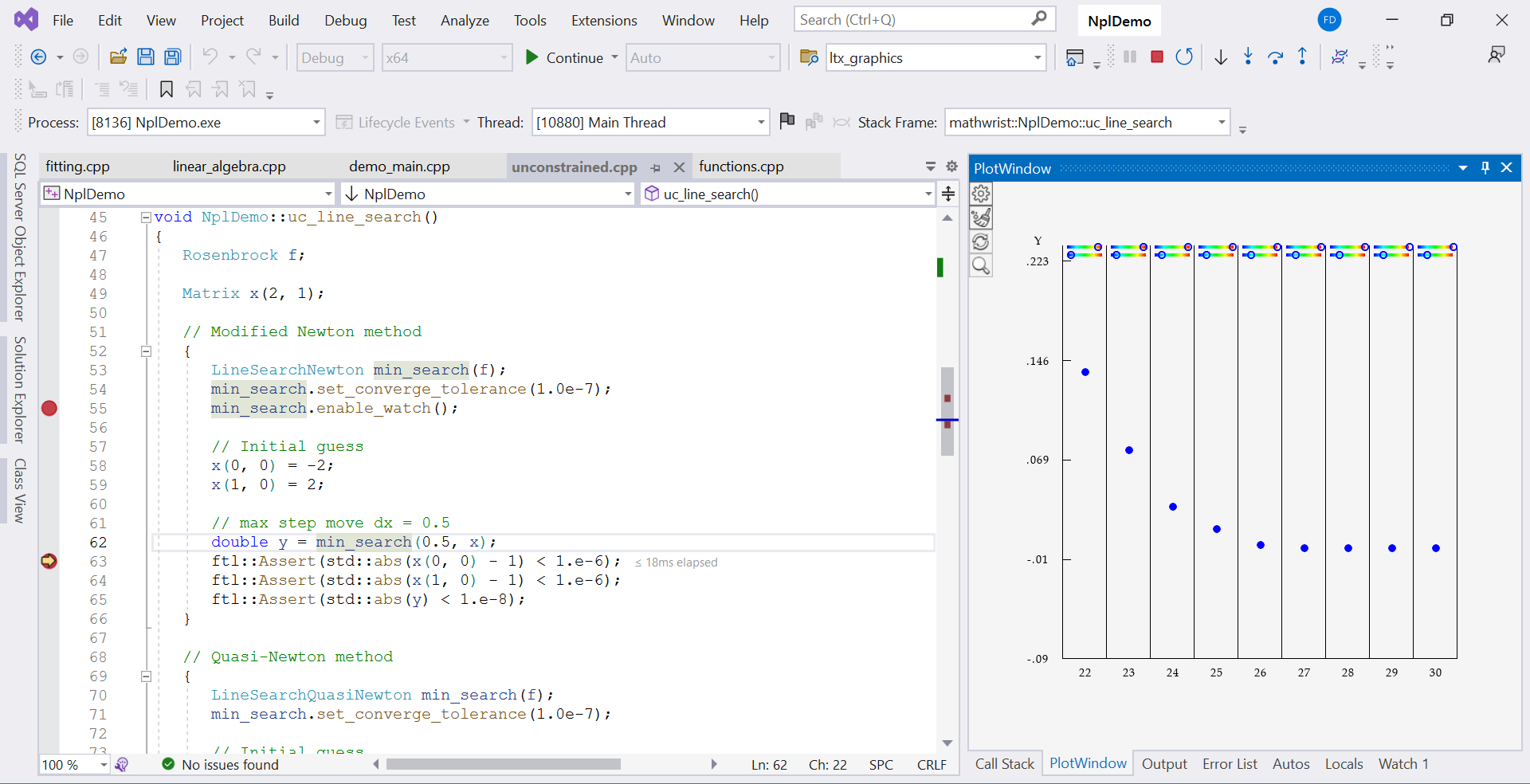
A single optimization frame is illustration in Figure 1. It corresponds to the second iteration of the optimization process (iteration number 2 pointed by the red arrow). The objective function value $f(x)$ at this iteration is represented by the blue dot (blue arrow annotation). Lastly, independent variable $x$ and its numerical range is represented by a small circle on a horizontal color gradient strip (shown in green arrow annotation). In this example the independent variable $x$ is 2-dimensional, hence we see two color gradient strips at the top of each frame. The location of a circle within its color gradient strip encodes the relative value of an independent variable $x_{i}$ within its numerical search range.

4 Animation Operations

When a dynamics animation is running, user can click the plot area to pause the animation. Click the plot area again will resume the animation. At any point of a dynamics display, users can right click the plot area to request GDE to immediately terminate the animation.

GDE Dynamics Plots Mathwrist User Guide Series