GDE Curve Plots
Mathwrist User Guide Series

(January 20, 2023)

Abstract

This document is a user guide of using Mathwrist’s Graphical Debugging Extension (GDE) tool to visualize curves, 2-d scatter data points and NPL math objects in Microsoft Visual Studio IDE. NPL is Mathwrist’s C++ numerical programming library. 2-d functions defined in NPL are directly recognized as plottable types in GDE. Please refer to our NPL documentation series for details. For an overview of GDE, please refer to our “GDE Overview” user guide.

1 Introduction

In this document, we focus on the GDE “Curve Session” and give details on plotting 2-d scatter data points, imposing a smooth curve fit to these data points and directly visualizing NPL 2-d math objects. It is recommended to first read our “GDE Overview” user guide in order to develop a high level understanding of GDE.

When an object is of a user defined matrix data type that has been exported to GDE as a part of plottable specification json file, GDE will further check if this matrix object has exactly 2 rows or 2 columns. If so, GDE will provide a choice to plot the columns of a 2-row matrix or the rows of a 2-column matrix as 2-d scatter data points. In addition, user may choose to plot the 2-d scatter pointer together with a smooth curve fit. We will illustate this feature in the next section by a walkthrough example.

When NPL is used in a user’s application, NPL matrix class mathwrist::Matrix, matrix views mathwrist::Matrix::View and mathwrist::Matrix::ViewConst are recognized as user-defined matrix types. Therefore 2-row or 2-column matrix objects and direct view objects can be plotted as 2-d scatter data points. Moreover, many concrete 2-d function and curve types defined in NPL can be added to GDE curve session for plotting.

2 Walkthrough Example

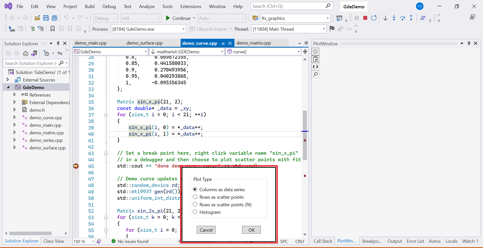
In this example code Listing 1, we populated some artificial data points $(x,y)$ from line 10 to 33, where $y=\sin(x\pi)+\epsilon$ , $x\in[0,1]$ for some random noise $\epsilon$ . We store these data points to a 2-column matrix sin_x_pi from line 35 to 41. Here sin_x_pi is a user-defined matrix type mathwrist::GDEDemo::Matrix, which we have exported as a consecutive memory matrix in our “mathwrist.gde.spec.json” file.

Listing 1: Curve Plot Example

2 #include <iostream>

3 #include <vector>

4 #include <random>

5 #include "demo.h"

7 void mathwrist::GDEDemo::curve()

8 {

9 // (x, y), y = sin(x * PI) + noise

10 static double _xy[] =

11 {

12 0, -0.049754564,

13 .05, 0.292976147,

14 0.1, 0.316827916,

15 0.15, 0.398965343,

16 0.2, 0.555522631,

17 0.25, 0.756583389,

18 0.3, 0.841009657,

19 0.35, 0.859861384,

20 0.4, 0.99532737,

21 0.45, 1.070343508,

22 0.5, 1.083259583,

23 0.55, 1.024642905,

24 0.6, 0.807780428,

25 0.65, 1.016032496,

26 0.7, 0.772325183,

27 0.75, 0.560368321,

28 0.8, 0.669872355,

29 0.85, 0.441580033,

30 0.9, 0.270493956,

31 0.95, 0.040293868,

32 1, -0.095356345

33 };

35 Matrix sin_x_pi(21, 2);

36 const double* _data = _xy;

37 for (size_t i = 0; i < 21; ++i)

38 {

39 sin_x_pi(i, 0) = *_data++;

40 sin_x_pi(i, 1) = *_data++;

41 }

43 // Set a break point here, right click variable name "sin_x_pi"

44 // in a debugger and then choose to plot scatter points with fit.

45 std::cout << "done demo case: curve" << std::endl;

47 // Demo curve updates with random noise over iterations

48 std::random_device rd;

49 std::mt19937 gen(rd());

50 std::uniform_int_distribution<> distrib(1, 10);

52 Matrix sin_2x_pi(21, 2);

53 for (size_t k = 0; k < 10; ++k)

54 {

55 for (size_t i = 0; i < 21; ++i)

56 {

57 double x = sin_x_pi(i, 0);

58 double eps = distrib(gen) * 0.01;

59 sin_x_pi(i, 1) = std::sin(x * std::_Pi) + eps;

61 sin_2x_pi(i, 0) = x;

62 sin_2x_pi(i, 1) = std::sin(2 * x * std::_Pi) + eps;

63 }

65 std::cout << "Break point here to plot updated curve." << std::endl;

66 }

67 }

After the data points are saved to sin_x_pi, we set a break point at line 45 and launch a debugging session. Right click variable sin_x_pi and choose “plot sin_x_pi” in context menu commands. Because sin_x_pi is a 2-column matrix, each row can be interpreted as a pair of $(x,y)$ data point. GDE will pop up a display choice window that includes “Rows as scatter points” and “Rows as scatter points (fit)” as illustrated in the red rectangle of Figure 1.

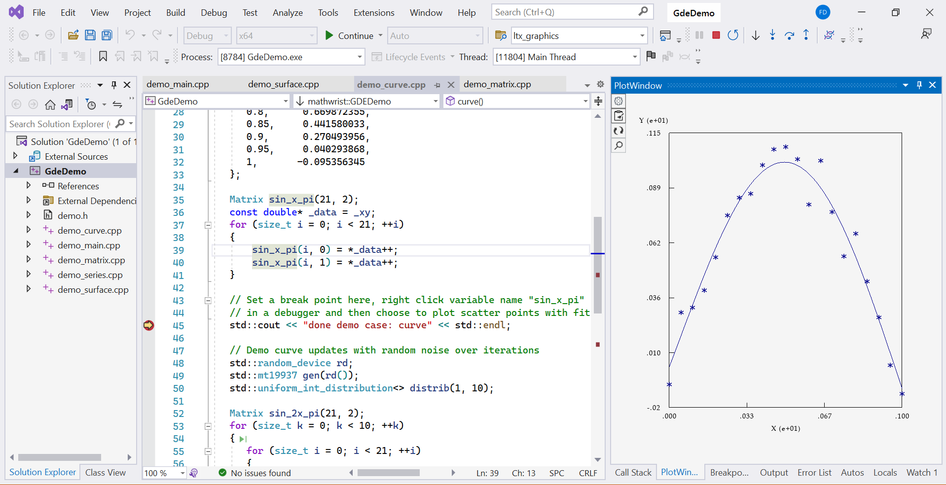
The left plot 2(a) in Figure 2 displays 21 $(x,y)$ scatter points corresponding to the radio button choice “Rows as scatter points”. The right plot 2(b) in Figure 2 is the result of choosing “Rows as scatter points (fit)”, which displays a smooth curve fitted to those scatter points.

Lastly, the code block from line 52 to 63 populates another set of scatter data points from function $y=\sin(2x\pi)+\epsilon$ and saves them to matrix object sin_2x_pi. We can add this object to the same plot and display it together with sin_x_pi as Figure 3.

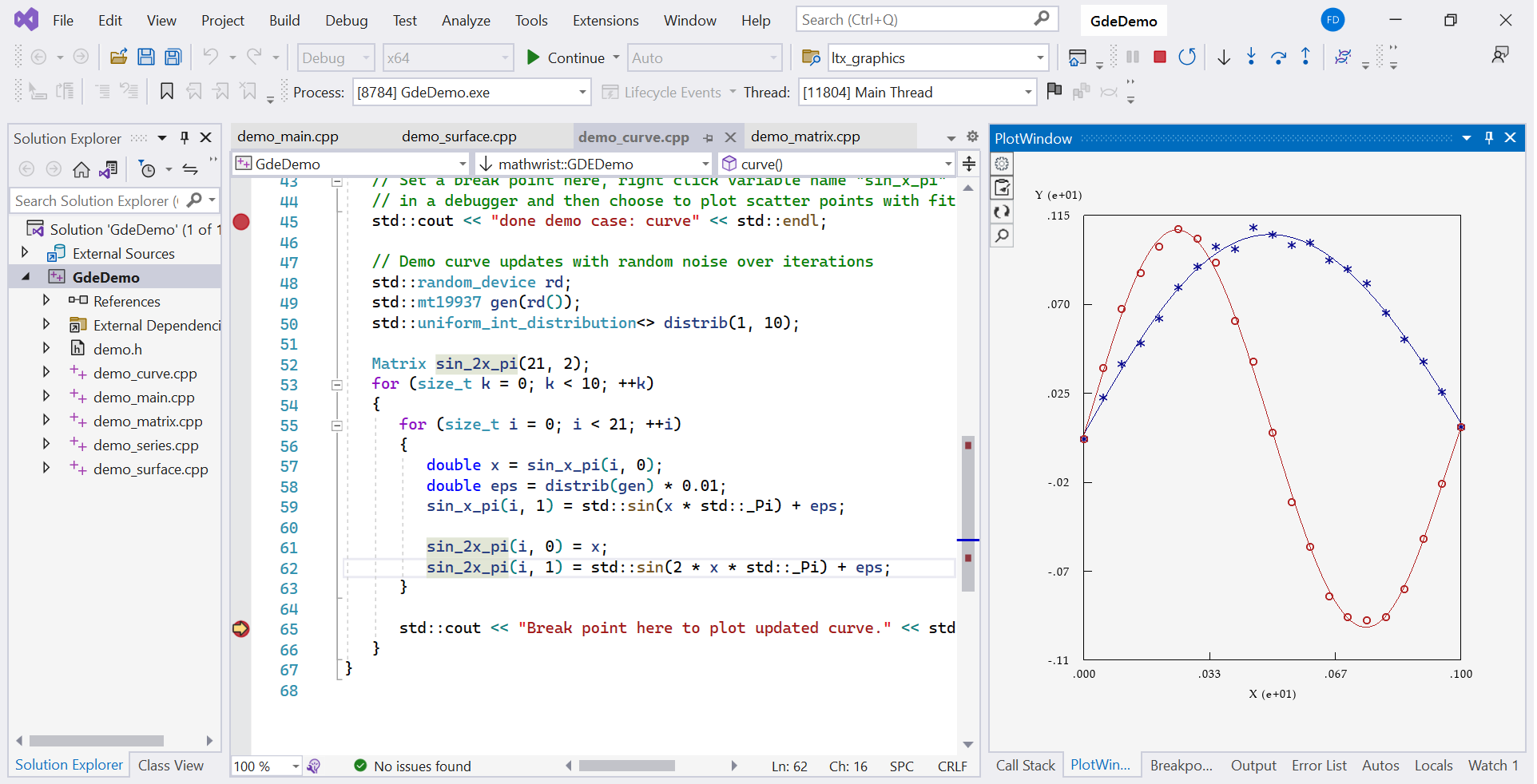
Figure 3: Curve Plot with Multiple Components

Note that we have adjusted the range of $y$ coordinate in display settings so that both sin_x_pi and sin_2x_pi fit in the same plot. Further, setting a break point i.e. at line 62, we can watch how these two objects are updated by random noise over iterations.

3 Session Management

Under the “Curve Session” tab in Figure 4, users can customize the display using the following UI controls.

•

Margin, set the display margin in the unit of pixels around the plotting area.
•

Axis $x$ min/max, set the $x$ axis range that function $f(x)$ is plotted.
•

Axis $y$ min/max, set the $y$ axis range that function $f(x)$ is plotted.
•

Font size, set the text font size on the curve plot.
•

Boxed, if selected, the plot area will display a solid line at each border.
•

Cancel, cancel the setting change.
•

Reset, reset the settings back to default values.
•

OK, plot the curve session using the current customized settings.

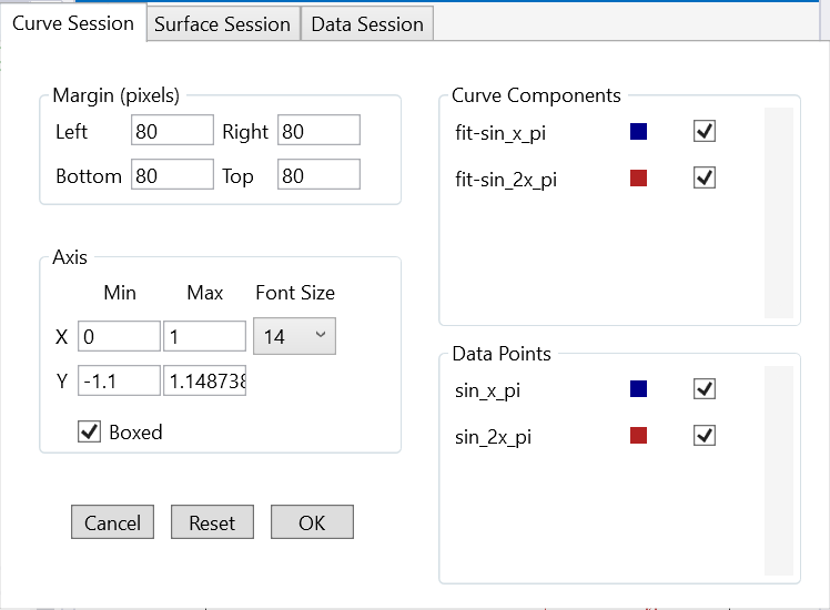
The right part of Figure 4 lists all curve components and scatter data points that have been added to the curve session. This component list has 3 columns, component name, color coding and selection checkbox. Note that the curve fit component name has a prefix “fit-” added to the variable name.

The checkbox control in component list section allows users to select which component is to be displayed together in the same plot. Check a curve fit component will automatically include its source data point component for display. Reversely, uncheck a scatter point component will automatically exclude its curve fit component from the display. Right clicking an individual component’s name will trigger a context menu “Delete” to delete this component from the curve session.

4 NPL Plottable Types

The following NPL C++ classes are recognized as 2-d plottables and can be added to GDE curve session for plotting.

•

mathwrist::FunctPiecewiseConst, a piecewise constant function.
•

mathwrist::FunctPiecewiseLinear, a piecewise linear function.
•

mathwrist::FunctPiecewiseLinearJump, a piecewise linear function that jumps at knot points.
•

mathwrist::BSplineCurve, a smooth curve that uses B-spline as basis functions.
•

mathwrist::InterpCubicSplineCurve, a cubic spline interpolation curve.
•

mathwrist::ChebyshevCurve, a smooth curve that uses Chebyshev polynomial as basis functions.
•

mathwrist::Matrix, mathwrist::Matrix::View and mathwrist::Matrix::ViewConst, a matrix or a direct matrix view that has 2 rows or 2-columns.

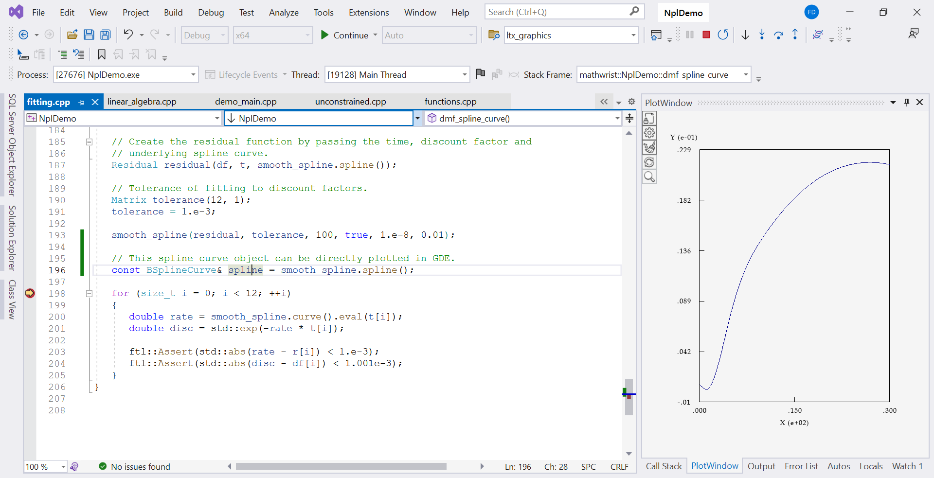
Figure 5 is an example screen shot of GDE curve plot in NPL’s demo project, where we have fitted a smooth mathwrist::BSplineCurve object. Right click the variable name spline of this object in Visual Studio debug session, and then click “plot spline” from debugging context menu. GDE then plots the curve in plot window at the right side of the IDE.