Data and Model Fitting
Mathwrist Code Example Series
Abstract
This document gives some code examples on how to use the data and model fitting features in Mathwrist’s C++ Numerical Programming Library (NPL).
1 Nonlinear Least Square
Assme a nonlinear model function with model parameters and . We have observed where for some random noise . The following example illustrates using modified Gauss-Newton method to recover model parameters from the observation data.
Note that the calibrated model parameters at line 90 and 91 are not same as the true parameters because we added some random noise to the observation data.
2 Model Fitting
This example is an application of smooth curve fitting in finance industry. In finance, it is a common practice to build a smooth interest rate curve that is a 1-dimensional function wrt time, i.e. . The discount factor at time is computed from a nonlinear function . In this toy example, we assume discount factors are observed from the financial market at a list of time points , i.e. for some data noise around 1.e-3.
The model fitting exercise here will use a cubic B-spline curve to represent the interest rate curve, , where is a vector of B-spline basis and is a vector of basis coefficients. Assume we choose B-spline knot points to be in time horizon. From the observed data , we want to recover the model parameter hence obtain a smooth interest curve.
We choose to build the curve by minimizing the curve roughness subject to discount factor fitting errors being within tolerance. In addition, we impose additional curve constraints to require the interest rates being positive at observed time points, i.e. .
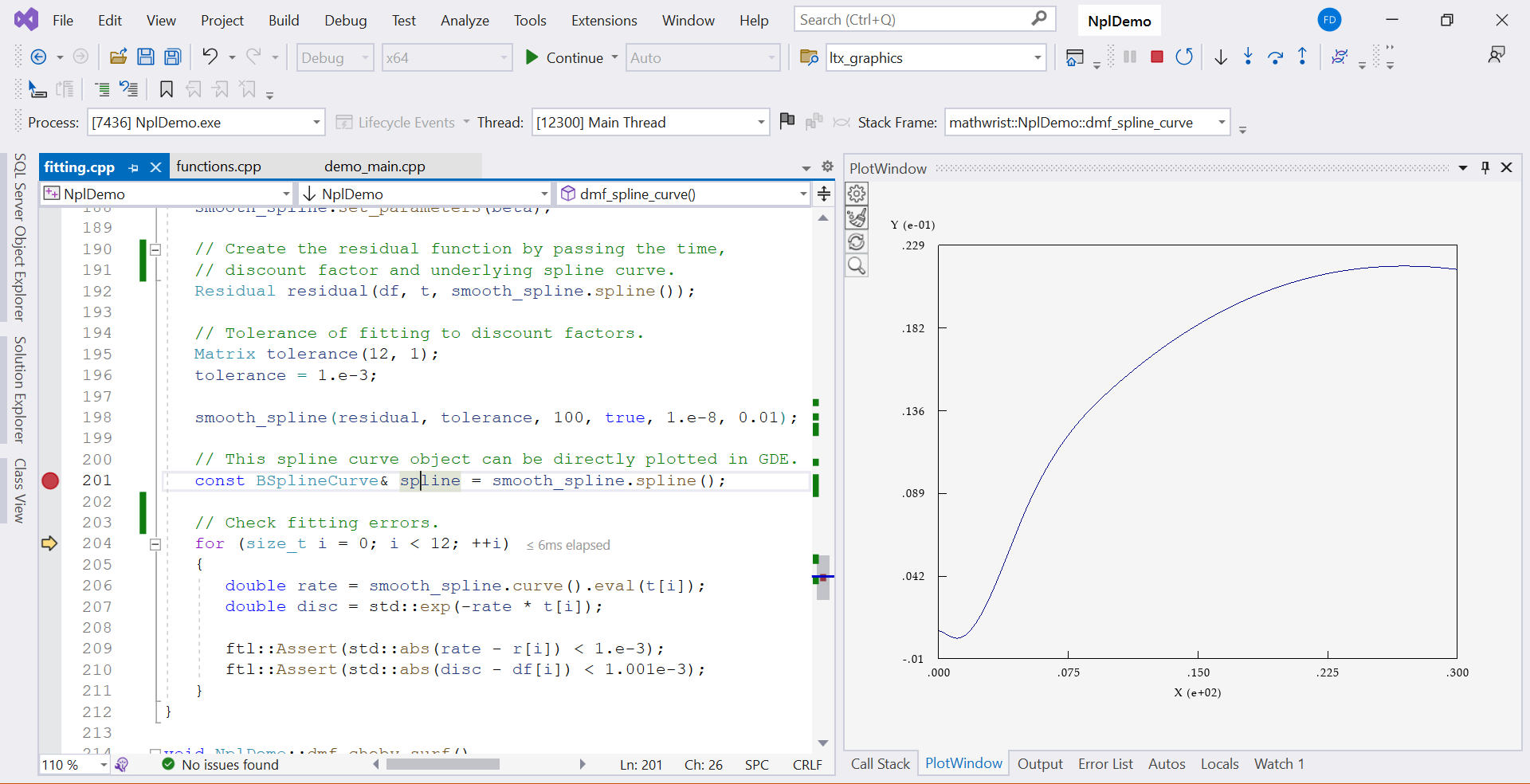
Note that at line 104, we set the discount factor fitting error tolerance to be 1.e-3, same magnitude as the noise that we artificially added to observation data. Setting the tolerance too small will be fitting to the noise. In practice, financial professionals have good knowledge on how tight market data should be fit.
After calibration, we can retrieve the smooth spline curve at line 109. This curve object is recogonized by GDE and can be plotted as illustrated in Figure 1.