Local Volatility Model Calibration under Optimal Control
Mathwrist White Paper Series

Abstract

High quality local volatility model calibration has always been a very challenging task in quantitative finance field. In this document, we present a high level overview of the PDE constrained optimal control technique that Mathwrist recently developed as a web application for commodity underlyings. This methodology can be readily applied to equities with minor modifications.

1 Introduction

Assume an underlying asset $S(t)$ follows the dynamics

$$\frac{dS(t)}{S(t)}=\mu (t)dt+\sigma (S,t)dW(t)$$ (1)

, where the local volatility function $\sigma (S,t)$ is deterministic. If $S(t)$ is a martingale in some risk-neutral measure, Dupire [1994] showed that the local volatility function satisfies a parabolic linear partial differential equation (PDE)

$$\frac{1}{2}{\sigma }^2(K,T)K^2\frac{{\partial }^{2}C}{\partial K^2}=\frac{\partial C}{\partial T}$$ (2)

, given European call option price $C(K,T)$ with maturity $T$ and strike $K$. In a more general setup where interest rate $r(t)\ne 0$ and $S(t)$ pays continuous dividend yield $q(t)$, e.g. $S(t)$ follows a SDE,

$$\frac{dS(t)}{S(t)}=(r(t)-q(t))dt+\sigma (S,t)dW(t)$$

, Gatheral [2006] gives a general form of the local volatility PDE using undiscounted European call option price,

$$\frac{1}{2}{\sigma }^2(K,T)K^2\frac{{\partial }^{2}C}{\partial K^2}+(r(t)-q(T))\left(C-K\frac{\partial C}{\partial K}\right)=\frac{\partial C}{\partial T}$$ (3)

The local volatility model is extremely useful in many ways. First, if the local volatility function $\sigma (K,T)$ is known, we can set the initial value $C(K,T=0)={(S_0-K)}^{+}$ and solve European call prices for all $T>0$ and all $K$ simultaneously. This is effectively a market making capability. In other words, one can quote the entire listed option market in terms of $\sigma (K,T)$.

Secondly, it can be shown that the local variance ${\sigma }^2(K,T)$ is a risk-neutral expectation of instantaneous variance conditional on $S(T)=K$ under T-forward measure. Local volatility surfaces can be used as the foundation to construct more complicated stochastic local volatility models for exotic derivative products.

Lastly, probably most importantly, for large option trading books and portfolio/risk management, the local volatility model is a consistent framework for option hedging and risk aggregation. In the traditional delta-hedge or delta-sigma-hedge, it is often tricky to decide what implied volatility should be used. Different practice, e.g. sticky delta, sticky moneyness, hedge ratio adjustments, vanna-volga etc could be very confusing even to professionals when context changes. They often are based on different assumptions and very likely introduce self-inconsistency if mixed together.

2 Existing Calibration Techniques

The most common practice to calibrate local volatility models currently perhaps is to first fit a smooth implied volatility surface, compute and differentiate European call prices using the implied volatility surface. This requires the implied volatility surface to be at least second order smooth. Small kinks on the implied volatility surface could be largely magnified in the local volatility surface hence produce unusable results. There are a variety of smoothing or smooth fitting techniques. Overall, it could be very challenging to fit a smooth implied volatility surface that perserves enough accuracy to match market quotes and yet is able to handle data noises. Most fundamentally though, implied volatility surface itself is not a mathematical model. It is not arbitrage free by construction. Additional care is necessary to prevent operable arbitrage opportunities.

PDEs (2) and (3) can be expressed in terms of implied volatility instead of call prices. e.g. Gatheral [2006],

$$\frac{\partial W}{\partial T}=V_L\left[1-\frac{y}{W}\frac{\partial W}{\partial y}+\frac{1}{4}\left(-\frac{1}{4}-\frac{1}{W}+\frac{y^2}{W^2}\right){\left(\frac{\partial W}{\partial y}\right)}^2+\frac{1}{2}\frac{{\partial }^{2}W}{\partial y^2}\right]$$ (4)

, where $V_L$ and $W$ are local volatility squared and implied volatility squared respectively, $y=\log (K/F)$ for forward price $F$.

Therefore alternatively, one can attempt to fit a smooth implied volatility surface and numerically differentiate using equation (4). But this is even tricker to do because equation (4) is highly nonlinear. Apart from nonlinearity, boundary conditions add extra difficulties if we want to numerically solve PDE (4).

It would be ideal to bypass the step of building an implied volatility surface and directly fit the local volatility model to market quotes. However, this could be an ill-posed “inverse problem” that generally leads to unstable calibration and delivers unexpected results. There seem to be very few works in the direction of solving an optimal control problem under PDE constraints. Mathwrist completed its first version of proof-of-concept work in 2023 and then developed a web application for user experience. Interested users are welcome to compare the performance of our web application to other methodology, particularly from the following aspects,

• Ability to handle large quote set.

• Calibration turnaround time.

• Accuracy to match the market.

• Shape of the local volatility surface and implied volatility smile produced from the model.

• Vulnerability to market data noise.

3 Commodity Local Volatility

3.1 Dynamics of Future Contracts

Specific for commodities, we assume a future contract $F(t,T_i)$ with maturity at fixed calendar time $T_i$ follows a SDE

$$\frac{dF(t,T_i)}{F(t,T_i)}=\alpha (t,F){\sigma }_{T_i}{\left[e^{-2{\beta }_1(T_i-t)}+{\lambda }^2{e}^{-2{\beta }_2(T_i-t)}\right]}^{\frac{1}{2}}dW(t)$$ (5)

Parameters ${\beta }_1\ge 0,{\beta }_2\ge 0$ are decay factors to produce Samuelson effect or humped volatility shape. Parameter $\lambda \ge 0$ can be interpreted as a blending factor between the two exponential functions. In the special case when ${\beta }_1=0$, ${\sigma }_{T_i}$ can be interpreted as the long term volatility and $\lambda$ behaves like a leverage factor on short term volatility. All together, ${\beta }_1$, ${\beta }_2$ and $\lambda$ determine the overall backbone shape of the vol term structure. These parameters are shared across all future contracts.

Parameter ${\sigma }_{T_i}\ge 0$ on the other hand is specific to the future contract $F(t,T_i)$. It is sometimes called the “big-T” parameter. And finally, $\alpha (t,F)$, sometimes referred as the “small-t” function, in our model setup is a local smile scaling surface that is also common across all future contracts maturing at $T_i,i=1,\mathrm{\cdots },n$. This small-t and big-T combined approach gives rich enough volatility dynamics in commodity derivative modelling.

3.2 Calibration of ${\beta }_1$, ${\beta }_2$, $\lambda$ and ${\sigma }_{T_i}$

Parameters ${\beta }_1$, ${\beta }_2$ and $\lambda$ can be calibrated from historical future prices. We take an alternative approach and fit them to the ATM implied volatility from all available future options. This step is carried out before we calibrate the smile scaling function $\alpha (t,F)$.

Now, consider a “reduced” model with flat smile for all futures,

$$\frac{dF(t,T_i)}{F(t,T_i)}={\sigma }_T{\left[e^{-2{\beta }_1(T_i-t)}+{\lambda }^2{e}^{-2{\beta }_2(T_i-t)}\right]}^{\frac{1}{2}}dW(t)$$ (6)

Note that here, we replace the contract specific ${\sigma }_{T_i},i=1,\mathrm{\cdots },n$ by a single parameter ${\sigma }_T$. Introducing a common parameter ${\sigma }_T$ for all futures facilates a stable calibration of ${\beta }_1$, ${\beta }_2$ and $\lambda$. These parameters determine the overall shape of the volatility backbone term structure.

Let $Y(t,T_i)=\log \left(\frac{F(t,T_i)}{F(0,T_i)}\right)$. For an option expiry , $Y(T,T_i)$ has the normal distribution $Y(T,T_i)\sim 𝒩(-\frac{\text{Var}(T,T_i)}{2},\text{Var}(T,T_i))$,

$$\text{Var}(T,T_i)={\sigma }_T^2\left[\frac{e^{-2{\beta }_1(T_i-T)}-e^{-2{\beta }_1{T}_i}}{2{\beta }_1}+{\lambda }^2\frac{e^{-2{\beta }_2(T_i-T)}-e^{-2{\beta }_2{T}_i}}{2{\beta }_2}\right]$$ (7)

Using the ATM option implied volatility quotes for all available option expiry, we construct a residual vector function $𝐫$ that measures the difference between market ATM volatility and model produced ATM volatility $\sqrt{\frac{\text{Var}(T,T_i)}{T}}$.

Let parameter vector ${\theta }^T=({\beta }_1,{\beta }_2,\lambda ,{\sigma }_T)$, we solve a constrained and regularized nonlinear least squared problem,

$${\arg }_{\theta }\min {\parallel 𝐫(\theta )\parallel }_2^2+\xi {\theta }^T𝐑\theta \text{s.t. }$$

$$-a\le {\beta }_1-{\beta }_2\le a$$

$$l\le \theta \le u$$

, where $\xi$ is a penalty factor determined by a generalized cross validation method. Matrix $𝐑$ is chosen in a way such that ${\theta }^T𝐑\theta$ somewhat measures the roughness of the backbone volatility term structure. Lastly, all constraint bounds are experimentally choosen.

Once ${\beta }_1$, ${\beta }_2$ and $\lambda$ are resolved, we discard the calibrated ${\sigma }_T$ value and proceed to determine the big-T parameters ${\sigma }_{T_i}$. It is a nature choice to choose ${\sigma }_{T_i}$ such that the backbone term structure exactly matches the ATM implied volatility at the terminal option expiry of each future contract. We actually find and take a more preferable way of choosing ${\sigma }_{T_i}$ that helps to better fit $\alpha (t,F)$ in the later stage of solving the optimal control problem.

3.3 Implied Volatility Smile

The backbone parameters are calibrated to ATM implied volatility from market quotes. Many exchange traded future options are American options. A “de-americanization” prerequisite step is involved to compute equivalent Black Scholes implied volatility from American option prices. There are various “de-americanization” techniques in practice, which by itself could be a separate subject. Here, we only focus on local volatility model calibration, assuming implied volatility are given.

Define the log moneyness variable $x=\log (F/K)$ at future price $F$ and strike $K$. We represent a smooth implied volatility curve by a $n$-degree Chebyshev approximation polynomial,

$$f(x)=\sum _{j=0}^n{T}_j(t(x)){\beta }_j$$

, where $t(x)$ mapps the selected log moneyness range to canonical domain $[-1,1]$ and ${\beta }_j$ is the coefficient of the $j$-th Chebyshev basis. Let $({\widehat{\sigma }}_i^{-},{\widehat{\sigma }}_i^{+})$ be the market implied volatility range at quoted strike $K_i$. We recover the set of basis coefficients $\beta =\{{\beta }_j\}$ by solving an elastically constrained quadratic programming problem,

$${\arg }_{\beta }\min {\beta }^T𝐑\beta \text{s.t. }$$ (8)

$${\widehat{\sigma }}_j^{-}\le f(x_j)\le {\widehat{\sigma }}_j^{+},\forall j$$ (9)

$$0\le f(x_{\text{lo}})\le u_{\text{lo}}$$ (10)

$$0\le f(x_{\text{hi}})\le u_{\text{hi}}$$ (11)

$$c_k\le f^{\prime \prime }(x_k)\forall k$$ (12)

First of all, our objective function (8) here is to minimize the curvature fluctuation on the implied volatility smile curve. The roughness matrix $𝐑$ therefore is constructed as

$${\beta }^T𝐑\beta ={\int }_{x_{\text{lo}}}^{x_{\text{hi}}}{f}^{\prime \prime \prime }{(x)}^2𝑑x$$

Secondly, for intraday quotes, the market volatility range in linear constraint (9) is taken from bid/ask. For settlement quotes, they could be taken as settlement quote minus/plus some tolerance. Due to market data noises, we impose the set of constraints in (9) as elastic constraints. If there is no feasible solution satisfying all these range constraints, we then solve an elastic programming problem. For the details of elastic constraints, please refer to our NPL product optimization white paper series.

Thirdly, constraints (10) and (11) are chosen to satisfy Lee [2003] implied volatility theoretical bounds at extreme strikes. Lastly, we impose curvature constraints in (12) to prevent the second derivative of the smile curve from being too negative. The iff arbitrage free condition along the strike dimension is to have a positive density $\frac{{\partial }^{2}C}{\partial K^2}$, implied from undiscounted European call option price $C$. When we express $\frac{{\partial }^{2}C}{\partial K^2}$ in Black Scholes formula wrt strike $K$ and apply chain rule to implied volatility from smile function $f(x(K))$, we can derive this butterfly arbitrage free condition as $f^{\prime \prime }(x)+c>0$ for some second order correction term $c$. Because of this correction term, it is necessary to require $f^{\prime \prime }(x)$ to be not very negative at least at some representative point $x_k$. The negative curvature lower bound $c_k$ at those points can be reasonaly estimated.

3.4 Normalizing the PDE

Both the original form of equation (2) and the general form (3) could be normalized to a “dimension-less” PDE. Define state variable $x=\log (F/K)$ and temporal variable $\tau =T_i-t$. We have tried two transformations of the undiscounted European call prices $C(T,K)$ to function: a) $v(\tau ,x)=\frac{C(T(\tau ),K(x))}{K}$ and b) $v(\tau ,x)=\frac{C(T(\tau ),K(x))}{\sqrt{F_{i}K}}$, used in Jackel [2013]. It appears that b) is slightly better. Then equation (2) then becomes to

$$\frac{\partial v}{\partial \tau }=\frac{1}{2}{u}^2(\tau ,x)\left[\frac{{\partial }^{2}v}{\partial x^2}-\frac{1}{4}v\right]$$ (13)

This transformation not only delivers better numerical performance but also brings the same initial value condition $v(0,x)={\left(e^{\frac{x}{2}}-e^{-\frac{x}{2}}\right)}^{+}$ to all future constracts. From the commodity dynamics (5), we have the local volatility as a control function

$$u(\tau ,x)=\alpha (t(\tau ),K(x)){\sigma }_{T_i}{\left[e^{-2{\beta }_1\tau }+{\lambda }^2{e}^{-2{\beta }_2\tau }\right]}^{\frac{1}{2}}$$

After all backbone parameters ${\beta }_1$, ${\beta }_2$, $\lambda$ and ${\sigma }_{T_i}$ are determined, we now want to recover the smile scaling function $s(\tau ,x)=\alpha (t(\tau ),K(x))$.

3.5 Optimal Control

Assume $s(\tau ,x)$ is parameterized by a set of control parameters $\theta$. From undiscounted European call option pricess $\{c_{i,j}\}$ at time to expiry ${\tau }_i$ and state $x_j$, we want to find $\theta$ such that the transformed option values $v({\tau }_i,x_j;\theta )$ are in bid-ask range. This imposes bounded constraints $c_{i,j}^{\text{bid}}\le v({\tau }_i,x_j;\theta )\le c_{i,j}^{\text{ask}}$. If we are working on settlement prices, the bounded constraints are $c_{i,j}-ϵ\le v({\tau }_i,x_j;\theta )\le c_{i,j}+ϵ$ for a tolerance setting $ϵ$.

In the space of control variables $\{\theta \}$ that produce $v(\tau ,x)$ according to the governing law in (13), which in turn satisfies the market price constraints, we like the local smile scaling function $s(\tau ,x)$ to be smooth. Choosing a smoothness objective function $\phi (\theta )$ suitable to the particular choice of $s(\tau ,x;\theta )$, our optimal control problem to recover $\theta$ can be loosely formulated as,

$${\arg }_{\theta }\min \phi (\theta )\text{ s.t. }$$

$$\frac{\partial v}{\partial \tau }=𝒜(v;\theta ),\forall \tau$$

$$c_{i,j}^{\text{bid}}\le v(\tau =T_i,x_j)\le c_{i,j}^{\text{ask}}$$

, where $𝒜(\cdot )$ is the spatial partial differentiation operator in equation (13). For example, if we solve this linear parabolic PDE (13) by finite difference method, at each time marching step from ${\tau }_l$ to ${\tau }_{l+1}$, the PDE constraint amounts to a linear equation ${𝐯}_{l+1}={𝐓}_l(\theta ){𝐯}_l$ for some finite difference matrix $𝐓(\theta )$ applied to the vector $𝐯$ of state function $v(\tau ,x)$ values at discretized states. Collecting all matrix vector multiplications, we obtain the final values of state function $v(T_i,x)$ as ${𝐯}_l={𝐓}_l(\theta ){𝐓}_{l-1}(\theta )\mathrm{\cdots }{𝐓}_0(\theta ){𝐯}_0$. Let $ℐ(𝐯)$ be an interpolation function on vector $𝐯$ to return the transformed call option values at quoted strikes. The concrete optimal control now is formulated as

$${\arg }_{\theta }\min \phi (\theta )\text{ s.t. }$$ (14)

$${𝐜}^{\text{bid}}\le ℐ\left({𝐓}_l(\theta ){𝐓}_{l-1}(\theta )\mathrm{\cdots }{𝐓}_0(\theta ){𝐯}_0\right)\le {𝐜}^{\text{ask}}$$ (15)

$$0\le s(\tau ,x)\le s_{\text{hi}}$$ (16)

$$c\le \frac{{\partial }^{2}s(\tau ,x)}{\partial x^2}$$ (17)

Constraint (16) requires the smile scaling function is bounded in a positive interval. Constraint (17) avoids the curvature of $s(t,x)$ being too negative.

Note that the PDE constraint (15) is a nonlinear implicit function wrt model parameters $\theta$. Mathwrist’s sequential quadratic programming solver is used to solve this optimal control problem. For the details of this solver, please refer to our NPL nonlinear programming white paper.

3.6 Sensitivity Calculation

The most crucial part of solving this optimal control problem is to efficiently and accurately compute the sensitivity $\frac{\partial }{\partial \theta }v(\theta ;\tau ,x_j)$. Bump and reprice technique is unacceptable in this context. Some observations will help the sensitivity calculation. First, taking differentiation operation wrt model parameters $\theta$ at both sides of equation (13) and rearrange terms, we have

$$\frac{\partial }{\partial \tau }\left(\frac{\partial v}{\partial \theta }\right)-\frac{1}{2}{u}^2(\tau ,x;\theta )\left[\frac{{\partial }^2}{\partial x^2}\left(\frac{\partial v}{\partial \theta }\right)-\frac{1}{4}\frac{\partial v}{\partial \theta }\right]=r(\theta )$$ (18)

$$r(\theta )=u(\theta ;\tau ,x)\frac{\partial }{\partial \theta }u(\theta ;\tau ,x)\left[\frac{{\partial }^{2}v}{\partial x^2}-\frac{1}{4}v\right]$$ (19)

So the sensitivities $\frac{\partial v}{\partial \theta }$ have the exactly same PDE coefficients as (13) except that they are inhomogeneous PDEs with the source function $r(\theta )$. A carefully implemented PDE solver should be able to solve both $v(\tau ,x;\theta )$ and $\frac{\partial }{\partial \theta }v(\theta ;\tau ,x)$ on the fly in the same process.

Secondly, applying differentiation operation to the chain of finite difference transformations, we have

$$\frac{\partial }{\partial \theta }\left[{𝐓}_l(\theta ){𝐓}_{l-1}(\theta )\mathrm{\cdots }{𝐓}_0(\theta )\right]=\frac{\partial {𝐓}_l}{\partial \theta }\left[{𝐓}_{l-1}(\theta )\mathrm{\cdots }{𝐓}_0(\theta )\right]+$$

$${𝐓}_l(\theta )\frac{\partial {𝐓}_{l-1}}{\partial \theta }\left[{𝐓}_{l-2}(\theta )\mathrm{\cdots }{𝐓}_0(\theta )\right]+\mathrm{\cdots }+$$

$${𝐓}_l(\theta ){𝐓}_{l-1}(\theta )\mathrm{\cdots }{𝐓}_1(\theta )\frac{\partial {𝐓}_0(\theta )}{\partial \theta }$$

If we choose $s(\tau ,x;\theta )$ such that $\theta$ has sensitivity locality in time, for example a sub set of parameters ${\theta }_1\in \theta$ has locality in $[{\tau }_0,{\tau }_1]$, then all above collapses to

$${𝐓}_l(\theta ){𝐓}_{l-1}(\theta )\mathrm{\cdots }{𝐓}_1(\theta )\frac{\partial {𝐓}_0({\theta }_1)}{\partial {\theta }_1}$$ (20)

This is just to solve the same PDE given a different initial value $\frac{\partial {𝐓}_0({\theta }_1)}{\partial {\theta }_1}$ subject to appropriate boundary conditions.

3.7 Accuracy and Speed

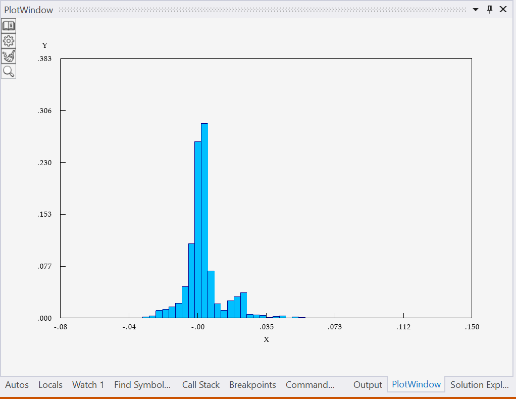
In the demo application, we calibrated the local volatility model to over 1400 WTI crude oil options across 10 different option expiry dates in 1.03 sec, details given in table 1. Row RMSE gives the root of mean square errors to market vol. Note that there are two numbers in this row. The RMSE for the first 7 option expiry is 0.0068. As the 8th to 10th option expiry add more data noise, RMSE goes up to 0.0117. The majority of the residual population is distributed within a very narrow range around 0 as shown in figure 1.

Machine	Lenovo Thinkpad X1 Yoga
Operating System	Windows 10 Professional, 64-bit
Processor	Intel(R) Core(TM) i7-6600U CPU @ 2.60GHz 2.81 GHz
Installed RAM	8.00 GB (7.83 GB usable)
Turnaround Time	1.03 sec.
RMSE	(0.0068, 0.0117)

Table 1: Test Report

Figure 1: Histogram of Residuals

References

- Derman and Kani [1994] E. Derman and I. Kani: Riding on a smile, Risk 7, 32–39, 1994
- Dupire [1994] B. Dupire: Pricing with a smile, Risk Mag., 7(1): 18-20, 1994
- Gatheral [2006] J. Gatheral: The Volatility Surface: A Practitioner’s Guide, Wiley Finance, John Wiley & Sons, 2006
- Jackel [2013] P. Jackel: Let’s Be Rational November 2013; Wilmott, pp 40-53, January 2015
- Lee [2003] R. Lee: The moment formula for implied volatility at extreme strikes, Mathematical Finance. Forthcoming.